RGB stands for Red, Green, and Blue. These are the “channels” in a color image. Each pixel has 3 numbers between 0 and 255 assigned to it.

• (255,0,0) red,
• (0,255,0) blue,
• (0,0,255) green,
• (255,255,0) yellow,
• (255,0,255) magenta,
• (0,255,255) cyan,
• (g,g,g) gray, for any g,
• (0,0,0) black,
• (255,255,255) white

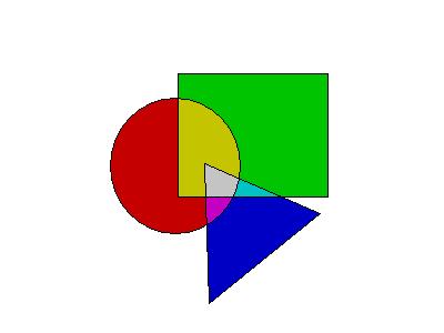
Every color image has three color channels - red, green and blue - and the image features you are after may be more pronounced with respect to one of them.

The channel-by-channel analysis allows one to consider each channel of the color image as a separate gray scale image and analyze them as needed. In Pixcavator just click a button in the Analysis tab for the channel you want.

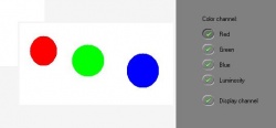
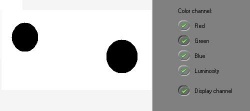
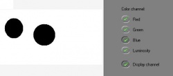
In the example below, the circles are of pure red, green, and blue. As a result, the red circle which is (255,0,0) becomes 255 in the red channel. But 255 is equivalent to white in this gray scale image. So the red circle disappears in the red channel. Similarly, the green circle will disappear if you choose the green channel, etc.

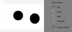
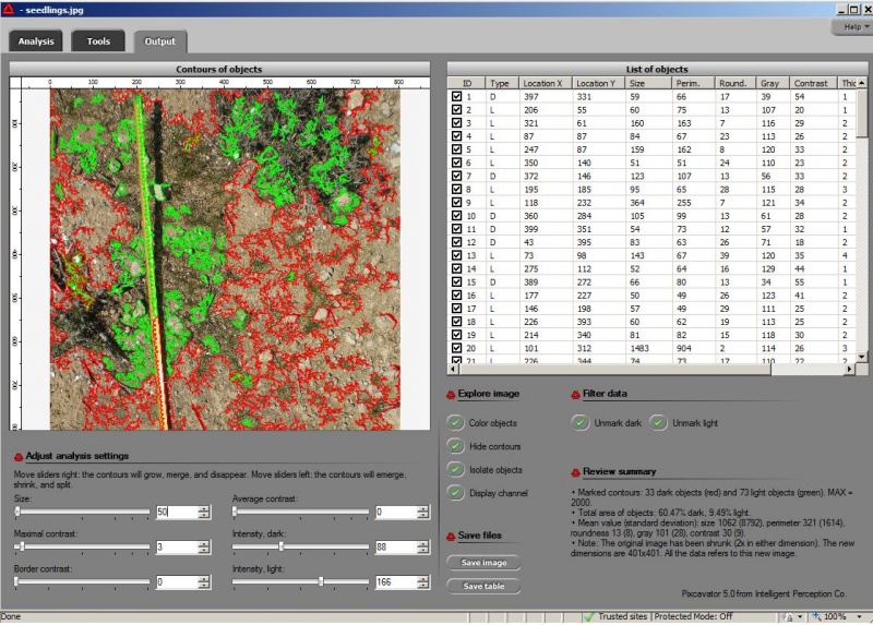
This option is important for some applications such as microscopy. Different features are sometimes better revealed in different channels. Below is the original image with two clear, to the human eye, features: red walls and green “cells”.

Read about analysis of this image here: http://inperc.com/wiki/index.php?title=RGB_channels.

Most of the recent content has come from two main sources. First, I have been adding, as before, examples of image analysis from the users of Pixcavator. The second is the course I’ve been teaching since last fall: Introductory algebraic topology. I plan to add more content from the courses that I teach: Vector calculus (this summer), Introductory differential geometry (next fall), and maybe also something of lower level like Calc1 (next winter).

What is the goal? I would like the site to cover a big chunk of the math curriculum, interlinked within and with the computer vision / image analysis topics (see The Mathematics of Computer Vision). Even though the format is identical to Wikipedia the presentation is very different. This is a textbook: more details, more examples, exercises, etc. It can still be used for reference.

The content comes directly from my lectures. I use Tablet PC with Windows Journal. I started doing this last fall and I really love the results: bright, colorful slides, but with the spontaneity and flexibility of a chalkboard. Later I transcribe the lectures into text, put it on the site, and simply copy the illustrations. (Plus, I don’t have to deal with chalk on my shoes, pants, and lungs!) I think this approach has huge advantages over the common practice of simply posting video lectures online: searchability, cross-linking, speed of download, the person can read and work at his own pace, etc.

Q: We need to “measure all the seedlings area (by dividing by the number of them I can get indication to their area and structure, and other parameters I can get)… The area covered is 80*80cm.”

The screenshot shows the results of my experiment. Here the red contours surround the darker areas (vegetation) and green surround the lighter areas inside. So, the total coverage is 60 - 9 = 51%. Unfortunately, I was unable to separate the seedlings from the rest of the vegetation.

There is also work with ecological researchers to measure vegetation coverage but mostly with horizontal shots.

Other examples of image analysis

Q: We “need to verify the internal diameter, external diameter and the wall thickness between the ID, OD and the reinforcement yarn. One issue we have is that the wall is not always concentric. We have a minimum wall thickness specification so we would like to measure the wall thickness at the thinnest point to determine if it meets our spec or not.”  

I analyzed one of the images. I found fairly good contours that capture the inner (red) and outer (green) borders of the hose with the settings that you can see in the screenshot. The measurements for this contours can be seen in the Pixcavator’s output table.

The area inside the red contour is 130,966. Assuming this is a circle, the area is equal to π*R², so the radius is

 R = √(130,966/3.14) = 204 pixels.

Then the external diameter is 408 pixels (one would have to do calibration at this point to convert to inches).

The area inside the green contour is 96,595. Assuming this is a circle, the radius is

 R = √(96,595/3.14) = 175 pixels.

Then the internal diameter is 350 pixels.

This suggests that the thickness of the wall should be 204-175=29 pixels. This is the average thickness of a ring with these measurements. To verify this number one can drop the assumption that these are circles and use the perimeters of the contours taken from the output table. Then

 average thickness
   = (area of the wall)/(average perimeter)
   = (130,966-96,595)/((1,547+1,283)/2)
   = 24 pixels.

A similar computation is presented here: Wall of a blood vessel.

Other examples of image analysis