Lengths of curves: theoretical aspects
The subject of lengths of curves in the digital envisonment has been discussed here several times. It’s summarized here: http://inperc.com/wiki/index.php?title=Lengths_of_curves. The main idea to take home is that no matter how high the resolution of your image is, the relative error of the measurement of the length of a “real” curve as approximated by a “digital” curve remains constant. That’s bad news for computing the perimeter or the roundness of an object in the image.

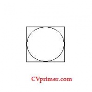
The perimeter of a square and that of the inscribed circle are the same.
A broader explanation for this failure is that the geometry of the universe is independent of direction, i.e. isotropic. By adding the grid and limiting our curves to it we make our approximation of this universe anisotropic. As the examples show, the horizontal and vertical directions are different from the rest. And no matter how much we improve this approximate universe by making the grid finer and finer, it will remain anisotropic. Choosing a triangular or hexagonal grid or other tricks won’t help.
The result is counter-intuitive. Indeed, refining the approximation has to lead to the exact result. Actually, there is a moment in calc1, when the issue arises and it requires some careful thinking.
The issue comes up when the definition of the Riemann integral is introduced. The integral is defined as the “limit” of Riemann sums, but what sums? They may be initially defined as a sums over intervals of equal length. In this case there is only one parameter and it may seem that you are just dealing with the same limits as the ones used for continuity, derivatives etc. However, this definition is inadequate if you want to prove some simple properties of the integral. Turns out, you need to be able to deal with arbitrary partitions of the interval. Then the Riemann integral is still a limit but a limit of Riemann sums over all possible subdivisions of the interval. For continuous functions it does not matter (you have to prove that), but for some other functions is does. These functions are non-integrable. The issue is often glossed over in a standard Calculus class (so that not to traumatize the students).
A similar situation here. We need to consider all possible rectangular grids. Then take the limit. The limit will be a two-parameter kind: the width of the pixel and its height go to 0, independently. Then, when both are smaller than some delta, the length of the approximated curve will be within some given epsilon from the length of the “real” curve. Problem solved!
Solved? It’s unclear how to use this insight to improve the accuracy…
Digital discoveries
- Casinos Not On Gamstop
- Non Gamstop Casinos
- Casino Not On Gamstop
- Casino Not On Gamstop
- Non Gamstop Casinos UK
- Casino Sites Not On Gamstop
- Siti Non Aams
- Casino Online Non Aams
- Non Gamstop Casinos UK
- UK Casino Not On Gamstop
- Non Gamstop Casino UK
- UK Casinos Not On Gamstop
- UK Casino Not On Gamstop
- Non Gamstop Casino UK
- Non Gamstop Casinos
- Non Gamstop Casino Sites UK
- Best Non Gamstop Casinos
- Casino Sites Not On Gamstop
- Casino En Ligne Fiable
- UK Online Casinos Not On Gamstop
- Online Betting Sites UK
- Meilleur Site Casino En Ligne
- Migliori Casino Non Aams
- Best Non Gamstop Casino
- Crypto Casinos
- Casino En Ligne Belgique Liste
- Meilleur Site Casino En Ligne Belgique
- Bookmaker Non Aams
- カジノ ライブ
- онлайн казино с хорошей отдачей
- スマホ カジノ 稼ぐ
- ブック メーカー オッズ
- Top 3 Nhà Cái Uy Tín Nhất
- Trang Web Cá độ Bóng đá Của Việt Nam
- Casino En Ligne Avis
- Casino En Ligne France
- Casino En Ligne
- 꽁머니 토토
- Casino Online Non Aams
- Meilleur Casino En Ligne


