Company
For photographers
For researchers
For developers
Image gallery
Blog

September 15, 2008

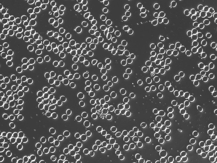
Image search engines still keep launching

Filed under: Image search, computer vision/machine vision/AI, rants — Peter @ 12:08 am

Last time I noticed that image-to-image search engines launch in batches was in May. Of course, “launch” usually means private beta. I also found it interesting that there are so many of them and yet they never mention or discuss each other.

Now, another batch - within a few days form each other.

First, Gazopa (what an awful name!) from Hitachi. Private beta.

Second, Imprezzeo. “Coming soon”.

Third, Picasa launched a face recognition feature. By most accounts it does not work well.

Fourth, VideoSurf “Unveils First Computer Vision Search for Video”. Private beta.

Finally, Idee updated its TinEye. Apparently, now it can match an image and its rotated version. That was my main problem with the application.

September 10, 2008

Counting fixed red blood cells: an image analysis example

Filed under: updates, image processing/image analysis software — Peter @ 8:23 pm

These are fixed red blood cells. The task is to count them with Pixcavator. They average 7.7 microns in size and were photographed unstained with differential interference contrast lighting. I had to crop the image to ensure reasonable processing times.


The quality of the image is good, but there is still a problem with the image. Each cell is captured by two light semicircles. These two semicircles aren’t connected to each other however (because the light comes from one direction?), so there are no full circles. The result is that cells can’t be treated as objects and they aren’t captured by the software. In the left image, there should be red contours for each of the cells like in the image on the right.


One way to get around this is to count the semicircles themselves (2 per cell). I ran Pixcavator with the following settings: 1000 for area and 100 for contrast.

The problem with counting semicircles is that many of some of them touch each other so that they form clusters. These clusters are what’s captured by Pixcavator. To deal with this problem I needed some extra computation that followed the analysis. In the last column of the saved spreadsheet (table below) I divided the areas of the clusters of semicircles by the area of one semicircle (“1030”). The total number of semicircles found this way was 35. Then the estimate was 17.5 versus 17 of manual count.

Another way to handle the problem is to start with some preprocessing. Erosion makes the light semicircles grow, they merge and form circular regions. Inside of those lie dark objects captured by Pixcavator. They correspond to cells.

I did 15 rounds of erosion (I had to use Pixcavator’s feature because ImageJ does erosions for binary images only). 15 is a lot as you can see.


Then I analyzed the image with the following settings: contrast 27, saliency 6768. The erosions, however, created several artifacts that had to be unmarked.

This method is more straightforward. With it, however, it is harder to get good results without manual intervention.

Live cells in the next post.

For other examples, see our wiki.

September 7, 2008

Gestalt and optical illusions

Another post about a book I am reading, From Gestalt Theory to Image Analysis. I want to write a few paragraphs about another interesting idea I found in the book.

Two Gestalt laws can be used to explain some optical illusions.

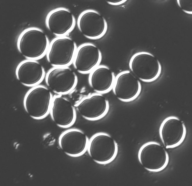
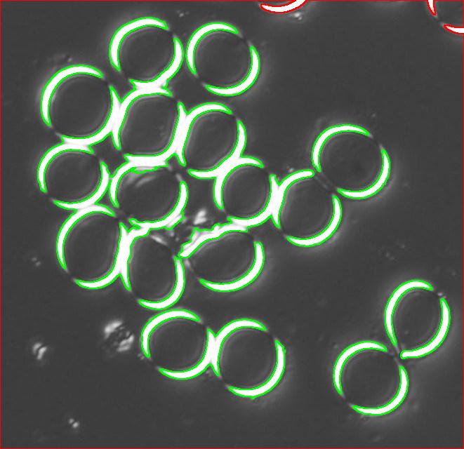
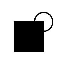
The amodal completion law: “[W]hen a curve stops another curve, thus creating a “T-junction”… our perception tends to interpret the interrupted curve as the boundary of some object undergoing occlusion.” This law is also related to the good continuation law.

Penrose triangle and fork are illusions (confusions?) are caused by the perceived depth in the image, locally:

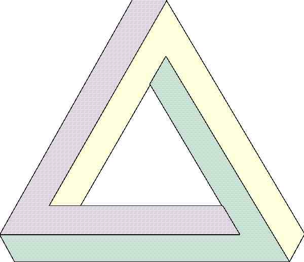
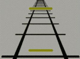
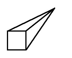
The perspective law: “Whenever several concurring lines appear in an image, the meeting point is perceived as a vanishing point (point of infinity) in a 3-D scene. The concurring lines are then perceived as parallel lines in space.” (Sounds reasonable, but how come all parallel lines are man-made?)

The Sander illusion (the left diagonal appears longer than the right one) and the Müller-Lyer illusion (the middle arrow appears longer) are caused by the perceived depth in the image:


I’d also add the Ponzo illusion (the “farther” bar appears longer than the “closer” one):

Also, remember Willy Wonka’s door?..

To summarize, both laws state that a person always sees 3D in a 2D image. But the fact is, one 2D image may correspond to many different 3D situations – including the drawing itself! That’s what causes the illusions.

So, these are interesting ideas that provide excellent explanations for the illusions. However, is it a good idea to try to design a computer vision system based on these laws? You don’t want to rely on a system that is so easy to fool

September 3, 2008

Measurement statistics of fibers: an image analysis example

Filed under: image processing/image analysis software, mathematics — Peter @ 5:11 pm

A few days ago I was contacted by a representative of a biotech company. He was interested in figuring out how Pixcavator can help them to automatically carry out a function that they currently do manually. They were looking for a method to automatically measure, document, and summarize characteristics of a certain kind of fibers in digital photos. Specifically, they needed: length and width, along with some very basic statistical data (size, length, width, ratio length to width, etc.), and graphical representations of the data (histograms). The image is below.

Capturing fibers wasn’t hard. Some of the irrelevant features are also captured but they were easy to filter out. The results would be better with better images: uniform dark background, less reflection etc. Separating fibers from each other would be a challenge; fortunately, the fibers were to be measured as “clumps” if they are attached to each other.

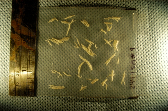
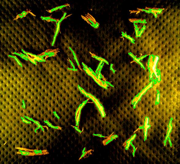
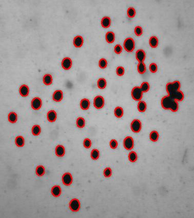
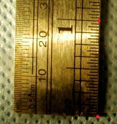
Averages are computed automatically but to have the answer in inches I had to calibrate the image. For that I used the ruler in the image (all the computations in the spreadsheet). I just found the end points of the one inch part of the ruler: from (193,235) to (196,44). This gives the distance

SQRT( (196-193) * (196-193) + (235-44) * (235-44) ) = 191 pixels.

So,

1 inch = 191 pixels.

Then I recomputed the averages. The result:

Average width: 0.02, average length: 0.52 inches.

This does not seem too far off. There may be a discrepancy in the way people understand width and length though. Basically, we consider the area and the perimeter of the object, then find the rectangle with these measurements, then take its width and length. Sometimes this is called the ribbon length.

The rest of the required output is easily acquired after some Excel work. The histogram of sizes (in pixels) of fibers is below.

For other examples, see our wiki.


| Home | Site map | Terms & Conditions | Contact us |                       Copyright© Intelligent Perception Inperc.com