On several occasions I was asked: Why wouldn’t we add a second slider to the size ruler? The logic is very convincing: “the first slider removes objects from analysis that are too small - with the second slider you can exclude objects that are too large”. There are real life problems that need this kind of analysis.
What is wrong with this idea? The problem is that the idea is “binary”. If the image is binary, excluding larger objects is a simple operation. We however deal with gray scale images. Sometimes objects in gray scale images look just like ones in binary images but often they have no well defined boundary. No well defined boundary – no well defined size!
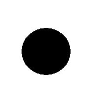
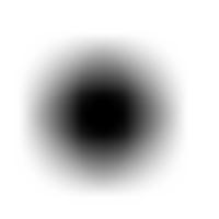
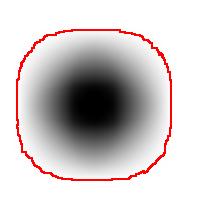
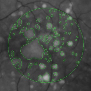
For example, this is a binary image of a circle and that is the same image blurred. There is clearly just one object here and it looks like circle. But what’s its size? It could be a small spot in the middle, or large circle, or it could be the whole image (why not?). If there are several objects like that, we can’t filter them based on larger/smaller comparison. As a result, we can’t even count them properly because without measuring we can’t tell noise from what’s important.
But wait a minute, of course, our software counts objects! So, how?
The user sets a lower bound on sizes of objects he considers important. Anything smaller is noise. What the user doesn’t know (but should) is what is an object. The definition of an object is in fact very simple:
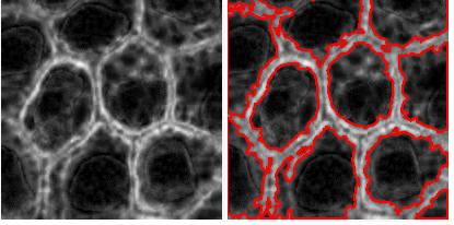
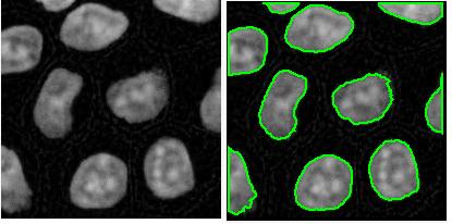
An object is either a dark region surrounded by lighter area or a light region surrounded by a darker area.
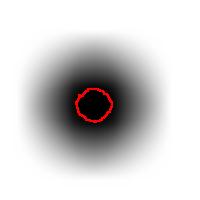
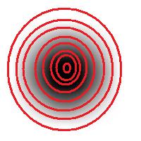
For example, in the above image we have many-many circular objects. Too many, in fact, because we know that there is only one! So, the objects that we’ve found aren’t actual objects but “potential” objects. At this point we need to select just one. How?
We use the bound chosen by the user! We exclude all potential objects that are smaller than this bound. Good, but even now we still have multiple objects. What do we do? We just take the smallest!
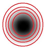
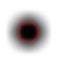
Roughly, once the bound is set, the object is allowed to grow until its size is over the bound.
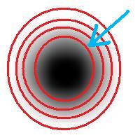
Suppose the bound is 100. Then what we present as the output is objects larger than 100 BUT as close as possible to 100. If the gray level changes very gradually, the objects’ sizes end up almost exactly equal 100. If this is the case, having an upper bound (say 200) in addition to the lower bound would not change the outcome…
That’s why only a single slider for the size is present. If object A is larger than object B, A is at least as important as B. A priori, all things being equal.
The second slider is for contrast and it operates in the exact same way: the object is allowed to grow until its contrast is over the bound. The logic is the same as before: a priori, if object A has a higher contrast than object B, A is at least as important as B.
OK, but what about those real life situations when you need to exclude larger objects? That’s when you turn from image analysis to data analysis. Of course, you’d have to make sure that you have captured all objects that you care about. That’s the hard part.
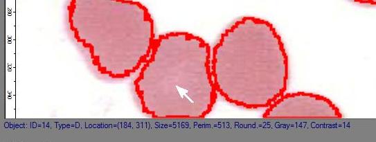
The data analysis stage is the easy part. If you have captured some noise or objects that you want to exclude, that’s OK. Now you simply filter the objects on the list based on any characteristic you want. Excel has plenty of tools for that. For example, the size is too large or too small. Or the perimeter, the contrast, the roundness, the intensity. Maybe you want only the objects from 100 to 200 pixels in size. Or maybe you are only interested in the objects within 300 pixels from the center of the image. All is easy at this stage.


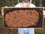 This came as a question from one of our users. The picture explains the problem: there is a bee frame with several hundred sealed brood. They are visible as tan hexagons (the dark circles are empty cells). Now, count them! Just like that – an outdoors photo taken with a regular digital camera, no registration, no calibration, etc.
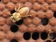 the image would need a higher resolution. If, however, the goal is just an estimate, Pixcavator can help. Then the task is less about counting and more about measuring… and some elementary school math.
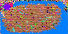
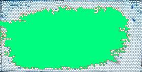
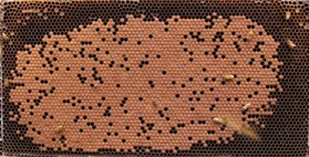


")


