August 31, 2008
I recently got a new book to read, From Gestalt Theory to Image Analysis, A Probabilistic Approach by Desolneux, Moisan, and Morel. I’ve heard of Gestalt before – apparently it’s a psychology theory of the mind. There is also an image analysis angle as Gestalt is a German word for “form” or “shape”. In the introduction the book presents are few Gestalt principles and gives them a mathematical interpretation. One principle I found especially relevant.
Werthheimer’s contrast invariance principle: Image interpretation does not depend on actual values of the gray levels, but only their relative values.
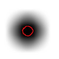
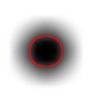
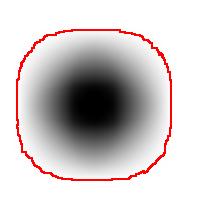
As the book further explains, the principle comes from the fact that one shouldn’t expect or rely on precise measurements of intensity. Once again this is our example:
 
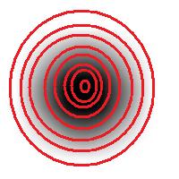
The second part of the principle suggests that one should look at the level sets of the gray scale function, as well as sub- and supra-level sets. In the blurred image above, the circle is still recognizable regardless of the low contrast. Which should be picked to evaluate the size of the circle is ambiguous however.
So far, so good. Unfortunately, next the authors concentrate on supra-level (or “upper level”) sets exclusively. This is a common approach. The result is that you recognize only light objects on dark background. To see dark on light will take an extra step (invert colors). Meanwhile the case of objects with holes (or dark spots on light objects) becomes really messy. Our algorithm builds the hierarchy of dark and- light objects in one sweep (see Topology graph).
The book isn’t really about Werthheimer’s principle but another one (more of a definition).
Helmholtz principle: Gestalts are sets of points whose (geometric regular) special arrangements could not occur in noise.
This should be interesting…
August 24, 2008
Previously we discussed the watershed algorithm for binary images. One thing that wasn’t explained was where the name comes from.
We start with the following approach. According to Gonzales and Woods: “we think of a gray scale image as a topological surface, where the values of f(x,y) are interpreted as heights.” This is good (except the redundant “topological”) and quite clear. Mathematically, if f(x,y) gives the value of gray of the pixel (x,y), we simply end up with the -graph of f (remember precalc?).
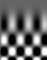  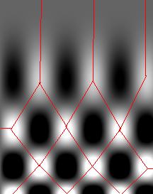
Next, we find the “catchment” basins. Mathematically, these are minimum points of the surface. However, to find basins’ borders we need to find the ridge lines that separate them. Mathematically, those are lines that go from one maximum point to another via the saddle points.
To summarize, we create a surface from the image by using the value of gray at a given pixel as the height of the surface above it. The light areas are the peaks and the dark areas are the valleys. Next, we flood the valleys, gradually. As we do that, we don’t allow the water to flow from one valley to another. How? By building dams. These dams will break the image into regions each containing a single valley. That’s image segmentation.
Let’s now take a look at the Wikipedia article: “The watershed algorithm is an image processing segmentation algorithm that splits an image into areas, based on the topology of the image.” First, any segmentation algorithm splits an image into areas. Second, any segmentation should be based on the topology of the image. So, what’s left is “The watershed is an image segmentation algorithm”.
The next sentence is “The length of the gradients is interpreted as elevation information.” Wait a minute, that’s not the same! The length of the gradient is the steepness of the surface. In the next sentence however the article seems comes back to the standard approach: “During the successive flooding of the grey value relief, watersheds with adjacent catchment basins are constructed.” And then again: “This flooding process is performed on the gradient image…” Using the gradient as the surface is an alternative approach to the watershed, so this must be a mix-up. Another approach is using the distance function for binary images.
We’ll discuss these issues in the next post.
August 20, 2008
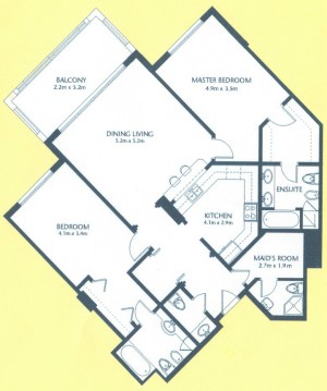 As a suggestion from one of our users, we used Pixcavator to analyze floorplans. The task is very simple – measure the rooms. As a suggestion from one of our users, we used Pixcavator to analyze floorplans. The task is very simple – measure the rooms.
Measuring irregular (or even regular) isn’t easy for a person because unless all rooms are rectangular one needs know some geometry. If the corners aren’t 90 degrees, you may have to measure them and then (OMG!) use trigonometry. The walls can also be curved. If the curves are known, all you need is calculus (OMG!!). It is unlikely that the formulas for the curves come with the floorplan, so digital image analysis seems inevitable.
The results are below. Of course, I had to “close” the doors first.
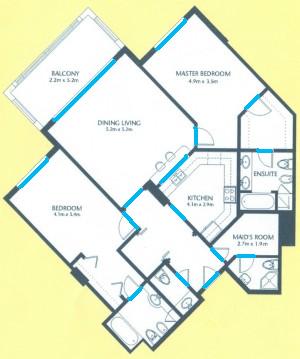 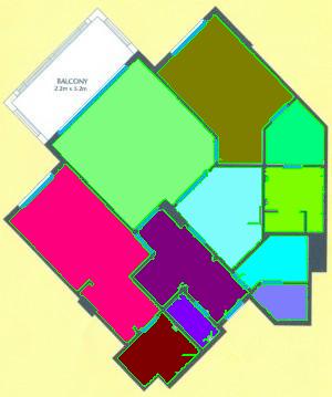
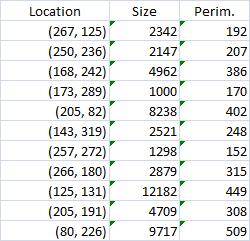
Calbration wasn’t addressed though.
August 17, 2008
The paper is A review of imaging techniques for systems biology (BMC Systems Biology 2008, 2:74) . Pixcavator is listed in “Table 2 - Overview of microscopy image analysis software” along with a few other companies/products. All the usual suspects are here: Image-Pro from Media Cybernetics, ImageJ, CellProfiler, Clemex Vision. The rest are less familiar and some of the companies are mostly about hardware. The paper itself is about imaging methods not image analysis. Even though this is not a endorsement by any stretch of imagination, it’s nice to be mentioned. (Smart people will also notice a few products that aren’t mentioned.) BMC stands for BioMed Central.
August 14, 2008
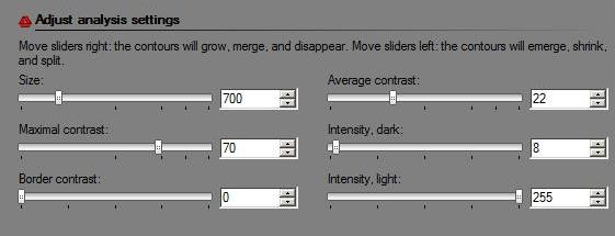
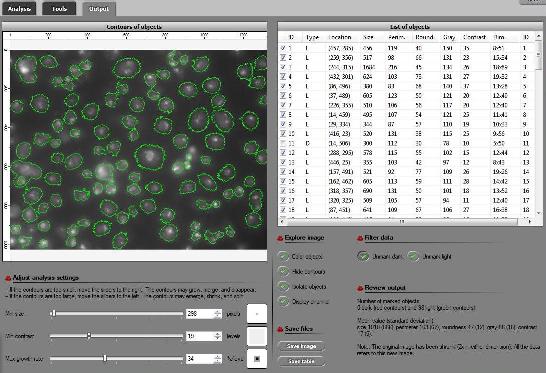
The updated interface is the first thing that you notice. All buttons and sliders are arranged in groups accompanied by headers. Text and tooltips were improved throughout.
The RGB channel analysis was completed to include all three channels. Just click a button in the Analysis tab for the color you want.
A new, “Max growth rate”, slider was introduced. Let me explain what it is. As you may remember object in the image are allowed to grow – from one level of gray to the next - up to the extent set by the slider. For example, the object will grow until it’s both larger than say 100 pixels and has contrast above 20. Now, this is a totally different kind of slider. If you choose 10, the object will be allowed to expand – from one level of gray to the next - as long as its size grows by 10% or less. Roughly, the expansion stops once the contour reaches a sharp edge. There will have to be more written about this after some testing. (To reproduce results you obtained with the older versions of Pixcavator just keep this value at 0.)
A new header is Data filtering. There are only two buttons here currently – Unmark dark and Unmark light. For convenience they were redesigned as follows. These are toggle buttons so that you can choose to concentrate on only, say, light objects without having to unmark dark every time you change the settings. There is more to come here.
The analysis summary now includes the mean values and standard deviations of all the main characteristics of objects (marked only).
The way contours are plotted was improved. Now red and green contours never overlap no matter how close they are to each other.
A noticeable speed-up was achieved, in both image analysis and graph analysis part. The memory usage was significantly reduced. There were also numerous minor improvements.
August 10, 2008
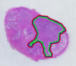
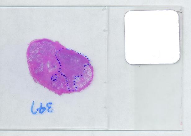 The first picture explains what normally happens when a prostate tumor has to be evaluated. The prostate is cut into thin slices and the slices are put on pieces of glass. Next, the doctor outlines the tumor within the prostate with a marker. Finally, the area of the outlined region is evaluated in each slice and the volume of the tumor is estimated. The first picture explains what normally happens when a prostate tumor has to be evaluated. The prostate is cut into thin slices and the slices are put on pieces of glass. Next, the doctor outlines the tumor within the prostate with a marker. Finally, the area of the outlined region is evaluated in each slice and the volume of the tumor is estimated.
Evaluating the area of the tumor with a naked eye will give you a very low accuracy. Best one can do to improve that is to superimpose a grid over the image and count the number of squares that fall into the tumor. Then the accuracy will be inversly proportional to the size of the square but the smaller the square the more complex the manual counting will be.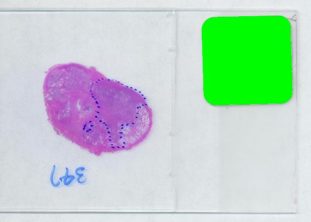
Digital image analysis is a necessity here.
I analyzed the shrunk version (615×439) of the image with Pixcavator followed by some back-of-the-envelope calculations.
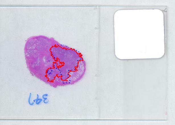
The critical part of analysis is the calibration. For that I used the square label in the image. It is known that its side is 2.2 cm. Now, I pushed the size slider almost all the way to the right and ended up with just one object -the label (green). Its area according to the table is 29,516 pixels. If we ignore the round corners (introducing some error here, unfortunately), it is a square. So 29,810 pixels = 2.2 * 2.2 = 4.84 sq cm.
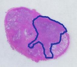
Next, the tumor. The dotted line is made solid using MS Paint. The you run Pixcavator. The contour has the area of 9,491 pixels. So, it is 9,491 * 4.84 / 29,810 = 1.54 sq cm.
 The end. The end.
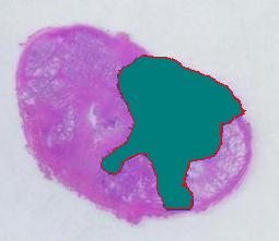
There is still the issue of error however. The error produced by hand drawing is estimated in the next experiment. Pixcavator evaluated the area on the outside of the curve (9,774) and on the inside (7,112). Hence the area of the curve is (9,774– 7,112) / 9,774 = 27% of the outside of the tumor. That’s the error.
It seems too high!
To verify the result, let’s approach from another direction. The perimeters are 542 and 530 respectively. Then the average thickness of the line is (9840-7342)/536 = 4.7 pixels. Examination of the image confirms this number. Of course, the error can be easily cut down by making the line 1/2 thinner but it will still remain high…
That brings us to the possibility of discovering the tumor within the prostate automatically. To be precise, the procedure would be semi-automatic not automatic, and it is the doctor who would make all the decisions. He chooses the contours and Pixcavator just counts pixels. What it gives you is a procedure that is somewhat simple – moving sliders until you have a good fit – and quite accurate – if the fit is good. Finding a good contour won’t require training but just a bit of practice. The last image shows that this approach isn’t totally unreasonable…
August 3, 2008
Image analysis and computer vision is the extraction of meaningful information from digital images. One of the most prominent application of computer vision is in medical image processing - extraction of information for the purpose of making a medical diagnosis. It can be detection and measurement of tumors, arteriosclerosis or other malign changes or it can be identifying and counting cells, etc. Other main areas are industrial machine vision (automatic quality inspection, robotics, etc) and the military (missile guidance, battlefield awareness, etc).
The science of computer vision consists of an abundance of image analysis methods. These methods have been developed over the years for solving various but often narrow image analysis tasks. The result is that these methods are very task specific and seldom can be applied to a broad range of applications.
Our conclusion is then that as a discipline computer vision lacks a solid mathematical foundation.
Our long term goal is to design a comprehensive computer vision system “from first principles”. These principles come initially from one of the most fundamental fields of mathematics, topology. The idea is that just as mathematics rests on topology (and algebra), computer vision should be built on a firm topological foundation.
Algebraic topology is a well established discipline within mathematics. Its main computational tools have been implemented as software (CHomP, Computational Homology Project, and others). However, this theory and these tools are only applicable to binary images.
A framework for analysis of gray scale images has been under development. It is called Pixcavator. It includes both an image analysis software and an SDK. Pixcavator was into a product that also includes image management and database capabilities.
Some further issues remain. Future projects include the development of:
- protocols for applying the framework for specific tasks (e.g., tumor measurement),
- new methods that resolve the ambiguity of the boundaries of objects in gray scale images,
- integration of the existing image analysis methods into the framework,
- a framework for video (first binary, then gray scale, etc),
- a framework for color images (and other multichannel images),
- a framework for 3D images (first binary, then gray scale, etc).
|
|
|


")


