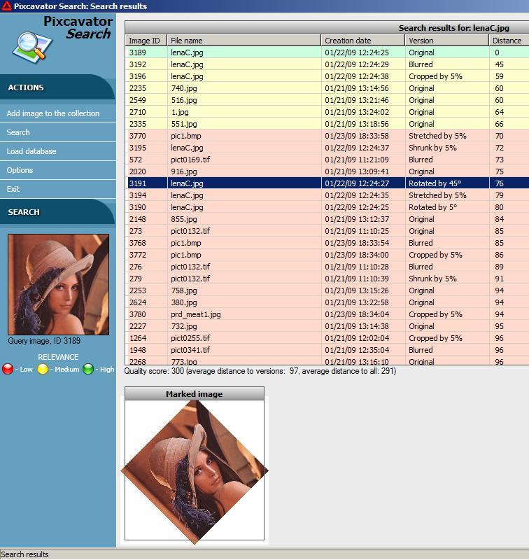
Over the last few months I have been contacted by many individuals and companies asking for help with their image analysis task or to evaluate the suitability of Pixcavator for them. I decided to pull some of these exchanges for my correspondence and present them to the public in the wiki under Image analyisis examples. The anonymity of the users is of course protected. There will be more examples.

From other news, I started to use Twitter (ID PeterSaveliev) to announce new posts for this blog as well as some short notes on the same subject. We’ll see how it goes… UPDATE: Boring!

I also decided to change, in part, how this blog is maintained vis-à-vis the wiki. In the past, a blog post would appear first. Then after a while, it would be turned into an article or articles in the wiki. Now I’ll start writing an article first and when it is sufficiently mature, I’ll post it in the blog. The news will appear as before.

I promised to update the article about Betti numbers in the wiki. So here it is.

Betti numbers count the number of topological features in the image.

For example, in the first image on the right the number of objects is 6, so the 0th Betti number B₀ is 6. The number of holes is 2, so the 1st Betti number B₁ is 2 as well.

More generally, the 0th, 1st and 2nd dimensional topological features are:

• objects or connected components – dimension 0,
• holes or tunnels – dimension 1, and
• voids or cavities – dimension 2.

These numbers in each dimension are captured by the Betti numbers, B₀, B₁, and B₂. Examples are in the table below.

	B0 (parts)	B1 (holes)	B2 (voids)
Letter O	1	1	0
Two letters O	2	2	0
Letter B	1	2	0
Donut	1	1	0
Tire	1	2	1
Ball	1	0	1

 

 The tire (torus) has two tunnels represented by these two “cycles”.

 

 This cycle is trivial and not to be counted.

In practice, i.e., computer vision and image analysis, you can’t count topological features. Instead you count “cycles” that capture them. Counting 0-cycles and 1-cycles in 2D is fairly simple.

Let’s now consider 1-cycles, i.e., circular curves, in 3D. In the torus, there are two kinds of cycles: the latitudes (one is red) and the longitudes (one is blue). The latitudes capture the tunnel inside the tire while the longitudes capture the tunnel through the tire.

Clearly there are many cycles that capture the same topological feature. So, how do you avoid overcounting them? The answer is: if two cycles are homologous to each other, they are counted as one.

One way to explain homology is this. Two cycles are homologous if they together form the boundary of a surface.

For example, any latitude is homologous to the red cycle because they are the two ends of a tube cut from the tire. Any longitude is homologous to the blue cycle because they are the two edges of a strip cut from the tire. This is why B₁ = 2.

In the sphere the blue cycle is homologous to a point, a trivial cycle, that’s why B₁ = 0. Another way to see that it is trial is to imagine how it can contract to a point like a rubber band. The same thing happens with the donut.

Betti numbers are combined together (as the alternating sum) to produce the well-known Euler number (aka Euler characteristics).

BTW, B_n = rank H_n.

In the previous post:

Recall = Number of retrieved images that are also relevant / Total number of relevant images.

Precision = Number of retrieved images that are also relevant / Total number of retrieved images.

In Pixcavator Search, the matches are simply ordered based on their distance from the query (just like Google). Then we need choose a cut-off. In the example considered last time, the cut-off was implicitly “all that fit in one page”. This is a reasonable standard for user oriented applications. For experimentation and testing, however, we may want to use the distance instead. For example, below I may choose the cut-off distance of 80: all images within 80 from the query are declared matches and retrieved, the rest are not. Then recall = 7/8, precision = 7/14.

The choice was made based on the examination of the search results for this particular image in an attempt to include as many as possible of “good” matches and, at the same time, to exclude as many as possible of the “bad” matches. More experimentation showed that 80 works OK for other queries as well. In general, however, this is not to be expected.

My conclusion is that the main drawback of precision and recall as a measure quality of the algorithm is that it requires a cut-off to separate the retrieved images from the rest. Then, the evaluation results depend on this choice. In fact, this measure ends up to be a measure of the quality of the query image, not the algorithm.

Technology News asks: “Will Microsoft’s Kumo Bring New Visual Dimension to Search?” and answers: “Microsoft seems to be amping up visual search capabilities in its upcoming Kumo search engine, if leaked screenshots are any indication.”

Well, they aren’t (see for yourself here). And neither is the leaked email.

The reporter seems to have been swayed by the CEO of Imprezzeo, a company offering their own image-to-image search engine.

Microsoft is certainly capable of doing that, e.g., Lincoln. Incidentally, Imprezzeo’s site has only a video demo.

In a recent post I discussed Pixcavator Search, prototype image-to-image software. As it searches for images based on similarity, a potential application of this software is a search for copyrighted images. With numerous application of this type out there, the discussion of performance evaluation is usually absent.

Let’s consider the performance evaluation commonly used in information retrieval. Below, we just replace “document” with “image”.

For a given query image, we assume the following:

• There are M relevant images in the collection = correct matches.
• When the query is executed, N images are retrieved.
• Out of those only R are relevant.

Then the following two measurements quantify the quality of the search:

Recall = R / M = Number of retrieved images that are also relevant / Total number of relevant images.

Precision = R / N = Number of retrieved images that are also relevant / Total number of retrieved images.

The recall is the answer to the question: How close am I to getting all good matches? The precision is the answer to the question: How close am I to getting only good matches?

In the example below, lenaC.jpg is the query and the program searched for its modified versions (7 modified versions of the original: stretched, rotated, noised, etc). Then N = 27, M = 8, R = 7, so recall = 7/8 and precision = 7/27.

Ideally, the value of recall and precision should each be equal to 1. However, in reality they go in the opposite directions. When the query is broad, the recall is high, but precision is low. When the query is restrictive, the precision is high and recall is low. We have all experienced this effect searching Google, Yahoo, etc.

But what does “restrictive” mean in the image search context? The query is an image, so what is a “restrictive image”?

Turns out that, for this particular algorithm, image with strong, distinctive features are best. This is certainly very vague. More specifically, these are images with large, high contrast objects. They should also have enough of these objects. For example, one large object, or several medium ones, or the whole image filled with dots. The last one isn’t something you’d call an image of good quality but it is very stable under noise, blur, and other transformations.

I’ll write some more on this. Meanwhile, this is the Wikipedia article about precision and recall. The article provides a probabilistic interpretation of precision and recall.