These are the new features in version 5.0.

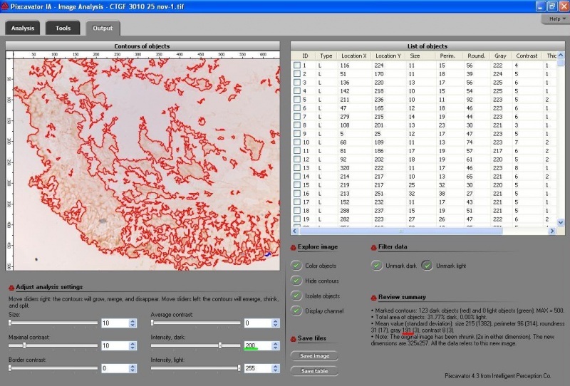
• Your choice of settings in the Output tab (the position of the sliders) is preserved when you load a new image to analyze.
• Your choice of color channels in the Analysis tab is preserved when you load a new image to analyze. With these two the user can apply the same settings to a sequence of images if they are similar in nature. So, we get as close as possible to bulk processing without actually creating this complex feature.
• Luminosity is a new color channel that you can choose. It is computed as a combination of the red, green, and blue values: 0.299*R + 0.587*G + 0.114*B. There are four channels now.
• “Display channel” is a new option in the Analysis tab (just like the one in the Output tab). If you have chosen to shrink the image, the shrunken version is shown. This way you can preview all channels and decide which is the best - before committing to time consuming analysis.
• The “Help” menu provides now the links to the help pages of this wiki. The user’s guide and the license are still provided with the program; they are to be found in the “Pixcavator” folder on your hard disk.
• The actual processing time is shown when it’s done, and a beep is produced - but only if processing has taken more than 5 seconds.
• Up to 2000 contours are now shown on the image and their statistics is also displayed. When there are more than 2000 contours, neither is shown.
• A few bugs have been fixed, some remain.

Download here.

Below is the abstract of a paper I am working on.

Suppose we have conducted 1000 experiments with a set of 100 various measurements in each. Then each experiment is a string of 100 numbers or simply a vector of dimension 100. The result is a collection of disconnected 1000 points (aka point cloud) in the 100-dimensional Euclidean space.

It is impossible to visualize this data as any representation that one can see is lim

ited to dimension 3 (by using colors one gets 6, time - 7). Yet we still need to answer the same questions about the object behind the point cloud: is it one piece or more? Is there a tunnel or a void? And what about possible 100-dimensional topological features?

This is a common approach to the problem.

For a point cloud in a euclidean space, suppose we are given a threshold r so that any two points within r from each other are to be considered “close”. Then each pair of such points is connected by an edge. If three points are “close”, we add a face, etc. The result is a cell complex (more precisely, simplicial complex) that approximates the manifold M behind the point cloud.

We want to count the number of topological features in M by means of the Betti numbers: the number of connected components in M, the number tunnels, the number of voids, etc. This information is contained in the homology of the complex.

Further, to deal with noise and other uncertainty one needs to evaluate the significance of these topological features. For each value of the threshold r we build a separate cell complex, then combine the homology groups of these complexes in a single structure, and count the features with a high measure of robustness. This measure, called persistence, is the length of the interval of values of r for which each of the topological features is present.

Even more important than these “global” properties may be the local topology of the data. For example, in both of the images above the datasets are 3-dimensional but what’s behind is 2-dimensional (surfaces). This is called dimensionality reduction.

Most of the links here are dead but the article will be fixed by the time I am done with the topology course.

A more detailed outline is here: Homological methods in manifold learning (warning: heavy math).

A new research paper that uses Pixcavator:

Adsorption Dynamics of CO on Silica Supported Gold Clusters: Cluster Size Effects in Molecular Beam Scattering Experiments by E. Kadossov, U. Burghaus (Department of Chemistry, Biochemistry, and Molecular Biology, North Dakota State University), link, published in Catalysis Letters.

From the paper:

“We report on particle size effects in the adsorption dynamics (gas-surface energy transfer) of CO, studied by molecular beam scattering… the effect of supported nano-size gold metal clusters on gas-surface energy transfer processes (adsorption dynamics)… For the statistical analysis, commercial imaging analysis software (Pixcavator IA 4.2) was used.”

There are nine, to the best of my knowledge, research papers that used Pixcavator and gave credit.

This edition is a version of Pixcavator that comes with a preloaded image. Which means that it’s not really a single program but many - one for each image.

It is a single file “exe” program that does not require any installation. As such it can be used as an alternative to screenshots, for demos etc.

This edition has all the features of the standard edition except for image processing tools. This way you can choose different color channels for your analysis, experiment with the sliders, and save your work.

Most of image analysis examples will soon have links to the corresponding files. For a start, try to run these two examples:

• immunohistochemistry,
• melanoma.

In FF: choose “Save”, then “Run”. In IE: just choose “Run”.

We will also be able to create such files as a service to our customers.

Q: “Immunohistochemistry was performed on my lung biopsies and now I have to analyse my staining. I would like to get a value for the colour intensity of my staining. … In the output of Pixcavator a mean value for grayness is given, but I don’t think all my brown staining is measured. Even if I adjust the threshold for size, not all objects are captured with a red or green contour.  ”

1. The difference in gray isn’t more pronounced because what is displayed is the average not the weighted average. So, one large dark object is outweighed by smaller, lighter ones. If you hover over objects (or look at the table) one at a time, you see a more noticeable difference. You can also save the data as a spreadsheet and compute the weighted averages. Certainly, if the difference is still too small, contrast enhancement would help.

2. It’s better to choose the green channel (or blue) than red. The features are much more distinct. If you click on “Display channel”, you’ll see the difference.

3. You are interested in dark objects only, red contours. So, the light ones only skew the averages. Click “Unmark light”.

4. The “Size” slider does not seem to reveal the features quite well. I used the simple thresholding instead, i.e., the “Intensity, dark” slider.

A screenshots is below. (This example may be somewhat similar: Measuring staining in the liver.)

More analysis here… 

Other examples of image analysis