This page is a part of the Computer Vision Wiki. The wiki is devoted to computer vision, especially low level computer vision, digital image analysis, and applications. The exposition is geared towards software developers, especially beginners. The wiki contains discussions, mathematics, algorithms, code snippets, source code, and compiled software. Everybody is welcome to contribute with this in mind - all links are no-follow.
Homology
From Computer Vision Wiki
Under construction...
Start with 2D Binary Images, Homology in 2D, and Topological Features of Images.
Cell decomposition of images is also necessary.
Linear algebra background is required.
Overview
Recall first the main principle of image decomposition:
In 2D we described 0- and 1-cycles as circular sequences of edges. We were able to get away with this informality because of the peculiarity of the 2D case. First, the boundaries of objects can be traversed sequentially. Also, unlike in higher dimensions, there are no “intermediate” dimensions. For the topological features of dimensions between 0 and the dimension of the image we will have to use a more precise mathematical description.
In the n-dimensional case, each frame is partitioned into a collection of regions: connected sets of black voxels and connected sets of white voxels.
- objects, blobs, or connected components are 0-cycles,
- holes or tunnels are 1-cycles, and
- voids or cavities are 2-cycles.
B0 B1 B2 homology
- Letter O 1 1 0 R, R, 0
- Two letters O 2 2 0 R2,R2,0
- Letter B 1 2 0 R1,R2,0
- Donut 1 1 0 R1,R1,0
- Tire 1 2 1 R1,R2,R1
- Ball 1 0 1 R1,0,R1
The boundary operator
This is where topology becomes algebraic topology. The relations between k-cells and their boundaries as combinations of (k-1)-cells are recorded by mathematical formulas. For example, if P is a pixel and E1, E2, E3, E4 are its edges then its boundary is
DP = E1 + E2 + E3 + E4.
Here DP, or D(P) if you prefer, is the boundary of P, so D is the boundary operator.
By the way, cells of all dimensions are easily recorded as lists of vertices:
- edge E = (V1, V2) is the list of its end points,
- pixel P = (V1,V2, V3, V4) is the list of its corners,
- voxel X = (V1, V2, V3, V4, V5, V6, V7, V8) is the list of its corners,
- etc.
Suppose that both the pixel P and its edges and E1, E2, E3, E4 are oriented clockwise, then
DP = E1 + E2 + E3 + E4.
But if pixel Q is oriented clockwise and its edges G1, G2, G3, G4 counterclockwise, then
DQ = – G1 – G2 – G3 – G4.
Suppose now that P and Q are adjacent, say, Q lies to the right of P. Suppose edges E1, E2, E3, E4 and G1, G2, G3, G4 go around each of the pixels starting from the left low corner. Then P and Q share an edge, in fact, E3 = G4. Then, we compute algebraically the boundary of the combination of P and Q:
D(P + Q) = DP + DQ
= (E1 + E2 + E3 + E4) + (– G1 – G2 – G3 – G4)
= E1 + E2 + E4 – G1 – G2 – G3
= E1 + E2 – G3 – G2 – G1 + E4.
Thus E1, E2, -G3, -G2, -G1, E4 go clockwise around P + Q, as expected.
Now, cells are combined into chains. For example, P and Q are 2-chains consisting of a single 2-cell each. Next, DP and DQ are 1-chains as sums of four 1-cells each. Thus, the boundary of a k-cell, such as E, P, or Q, or a k-chain, such as P + Q, is a (k-1)-chain. Here’s another example: DE = V2 – V1.
Moreover, both DP and DQ are “closed” 1-chains in the sense that the 1-cells form a circular curve. Such chains are called cycles. However, DP and DQ are trivial 1-cycles in the sense that they are boundaries of 2-chains, P and Q. We are interested in nontrivial cycles such as C and C’. They represent holes in the image.
Further exposition of homology theory is postponed until later, but it suffices to say that the topological features in the image are found as cycles of appropriate dimensions. Since algebraic topology is a highly developed and mature theory, all results are mathematically proven.
Exercise 1 Compute D(P – Q). Compare to D(P + Q).
Exercise 2 Compute DC, DC’, D(C + C’). What is DK if K is any cycle?
Exercise 3 Compute DDP. Draw conclusions. Answer
Cycles and homology classes
Recall that cells of all dimensions are recorded as lists of vertices:
- edge E = (V1, V2) is the list of its end points,
- pixel P = (V1,V2, V3, V4) is the list of its corners,
- voxel X = (V1, V2, V3, V4, V5, V6, V7, V8) is the list of its corners,
Cells are combined into chains. For example, …
Now, DP is a “closed” chain in the sense that its 1-cells form a circular curve. Such chains are called cycles. A cycle C is easy to identify because DC = 0. However, DP and DQ are trivial 1-cycles in the sense that they are boundaries of 2-chains, P and Q. We are interested in nontrivial cycles such as C and C’. They represent holes in the image.
As before, each frame is partitioned into a collection of regions: connected sets of black pixels and connected sets of white pixels. Beyond that, higher dimensional cycles that represent the homology classes of the image are used. These cycles are constructed through an incremental process as cells, one by one, are added to and removed from the current frame to transform it into the next or adjacent frame.
The previously described algorithm is extended to process nD cell complexes (simplicial, cubical, geometric, or CW-). In general, cell complexes are made of cells that can have an arbitrary number of faces of all dimensions and different shapes. It is assumed that a k-cell is homeomorphic to a k-ball. Thus, a k-cell is a k-dimensional polygon, possibly curvilinear, together with its orientation, i.e., the order of vertices. Further, k-cells are attached to each other only along their boundaries, which are made of (k-1)-cells. As a result, the cell decomposition of the frame is a directed graph of cells with arrows pointing from a k-cell to all of its (k-1)-faces.
Partition is now just a part of a more general topological decomposition of the image.
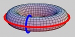
Consider the picture of the torus. The goal is to capture the tunnel that goes along the tire. However, the tunnel is impossible to see if you are standing on the surface. The reason is that the only information you have is how these cells are attached to each other. The only way to capture it is by considering the cycles that go around it. The problem is that for just one tunnel there are infinitely many of such cycles. For example, every “meridian” goes around the tunnel, not just the blue one. The answer to this problem is to say they are all equivalent, or “homologous”, and they are counted as one. These cycles are indeed homologous (similar) as one can be slid to another along the surface, while the blue and the red are not. Algebraically, this works as follows.
The version of the method that we present is for the homology groups over any “field” such as R or {0,1}. Suppose we are given a frame of the image. A k-homology class in this frame is represented by a chain of k-cells that can be recorded as an M-vector, where M is the total number of k-cells in the frame. As an illustration, a component of this vector is 1 if the corresponding cell is present, -1 if it present with the opposite orientation, 0 if it is absent.
The k-boundary operator D is an M×N matrix where N, the number of rows, is the total number of (k-1)-cells in the frame. Then the boundary of a chain C is the matrix product DC. By means of D, it is easy to verify whether any two k-chains A and B are homologous: the difference between them is the boundary of a (k+1)-chain T: A – B = DT. The existence of T is verified by the standard linear algebra techniques. In this case, A and B belong to the same k-homology class H=[A]=[B].
Examples of A and B are: two vertices in the same component of any cell complex (k=0); two meridians of a torus, but not a meridian and the equator (k=1); the inner surface and the outer surface of a thick sphere (k=2).
These chains are cycles: they have zero boundaries, DA=0. They are also “nonzero”: they are not boundaries of (k+1)-chains. They can be justifiably called “holes”. Each homology k-class can be represented by one of its k-cycles. The algorithm maintains a list of cycles the homology classes of which generate the homology group. These cycles will be called homology generators or simply generators.
There will be more here...
Continue to Homology software
Digital discoveries
- Casinos Not On Gamstop
- Non Gamstop Casinos
- Casino Not On Gamstop
- Casino Not On Gamstop
- Non Gamstop Casinos UK
- Casino Sites Not On Gamstop
- Siti Non Aams
- Casino Online Non Aams
- Non Gamstop Casinos UK
- UK Casino Not On Gamstop
- Non Gamstop Casino UK
- UK Casinos Not On Gamstop
- UK Casino Not On Gamstop
- Non Gamstop Casino UK
- Non Gamstop Casinos
- Non Gamstop Casino Sites UK
- Best Non Gamstop Casinos
- Casino Sites Not On Gamstop
- Casino En Ligne Fiable
- UK Online Casinos Not On Gamstop
- Online Betting Sites UK
- Meilleur Site Casino En Ligne
- Migliori Casino Non Aams
- Best Non Gamstop Casino
- Crypto Casinos
- Casino En Ligne Belgique Liste
- Meilleur Site Casino En Ligne Belgique
- Bookmaker Non Aams
- カジノ ライブ
- онлайн казино с хорошей отдачей
- スマホ カジノ 稼ぐ
- ブック メーカー オッズ
- Top 3 Nhà Cái Uy Tín Nhất
- Trang Web Cá độ Bóng đá Của Việt Nam
- Casino En Ligne Avis
- Casino En Ligne France
- Casino En Ligne
- 꽁머니 토토
- Casino Online Non Aams
- Migliori Casino Non AAMS
- Meilleur Casino En Ligne
- Casino En Ligne France Légal
- Casino En Ligne France Légal
- Casinos En Ligne
- Mejores Casinos Online
