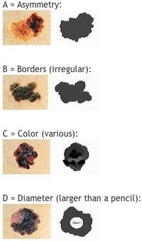
Recall the detection is based on the mnemonic ABCDE:

• Asymmetry of the spot.
• Border: irregular.
• Color: varies.
• Diameter: large.
• Evolution of the spot.

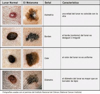
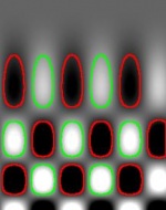
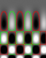
The test for asymmetry was discussed in the last post. Suppose it is passed: the spot is symmetric more or less. Now, what about the border? To fail B, it is supposed to be irregular. Is it possible to be irregular and symmetrical at the same time? Yes, if the curve has large, but not repetitive, oscillations on one side of the axis of symmetry and then has the same oscillations on the other side. The larger are these oscillations, the less likely this is to happen however. A more likely possibility is a lot of small oscillations. In other words, we’d have to zoom in on a piece of the border and measure the smoothness of the curve. How isn’t obvious. The difficulty is that no digital curve is smooth. So, we’d have to look for oscillations that are small enough to be feasible and large enough not to be confused with edges of pixels…

Next is the color. Most normal moles are uniform in color. But varied shades of brown, tan, or black may be a sign of melanoma. Since all of the colors are close to each other in the spectrum, it’s possible that analysis of the gray scale would suffice. In that case the variability of color is easy to capture by computing the standard deviation.

The test for the diameter reads: a mole smaller than a pencil eraser is probably not cancerous. It is unclear whether the diameter (it fits in the mnemonic so well) is to consider here or the size/area is just as good. Either way it’s simple and reliable.

Finally, the evolution of the spot: “the change of a spot may indicate that the lesion is becoming malignant”. Not indication what kind of change that would be. The best guess is: the change of any of the other 4 characteristics.

In spite of their vagueness, these tests can be developed into image analysis procedures - with a help of medical experts. Next one would need to get from this string of numbers to a diagnosis or at least a score that reflects the likelihood of cancer. This step would also require input from a medical expert, though machine learning would be tempting too, for some…

This will be filed under Measuring objects in the wiki.

Melanoma is a kind of skin cancer so common and obvious at the same time that doctors encourage self-detection, even on TV, which is unusual. The detection is based on the mnemonic ABCDE:

• Asymmetry of the spot.
• Border: irregular.
• Color: varies.
• Diameter: large.
• Evolution of the spot.

There are many images out there that illustrate these features but the one above is one of very few I could find that compares benign lesions to cancerous ones. E is missing which is not uncommon.

The tests seem so simple, it’s tempting to try to design an image analysis system that would detect this cancer. Even though it’s been probably done before, let’s see how far we can go within the limits of a single blog post.

There is clearly an overlap between A, B and D. I will try to separate them as much as possible.

A for Asymmetry: How do we detect that by image analysis? On the face of it, this is about the measure of symmetry of the spot. If this is the case, the simplest approach is the following. Find the major axes of the spot, then carry out reflections about these axes and compute the overlap of the resulting spots (3 total) with the original. The overlap should be computed in relative terms in order to separate A from D.

Of course to detect even more symmetry one need to look at all rotations but that may be unnecessary.

Another, even simpler, approach is to compute the roundness of the spot as “[m]ost moles - the kind you usually don’t have to worry about - are more or less round.” That may have to be preceded by smoothing the border (Gaussian blur or similar) in order to separate A from B.

Either approaches has its problems: the major axis are badly affected by noise while computing the roundness produces errors even without noise.

To be continued…

Previously we discussed the watershed algorithm – and we examined where the name comes from. Suppose we have a function f(x,y) and a surface that is the graph of f.

Next, we flood the valley and build dams so that we don’t allow the water to flow from one valley to another. These dams will break the image into regions each containing a single valley.

In the standard settings when f(x,y) is the gray level (in the example on the right f(x,y)=sin(x)sin(y)), what is captured by these dams are the dark spots. Then the light areas are the peaks and the dark areas are the valleys. Then, for example, if you have an image of dark cells on a light background, you’ll have the cells enclosed inside these regions.

What if the cells are light and the background is dark? Then you’ll have to turn everything upside down. For example, you can replace the surface given by f(x,y) with the one given by 255-f(x,y). Not a problem but inconvenient. Why? Because you have to tell your program what you are looking for: light on dark or dark on light. It is better if you don’t have to use a priori information so that the analysis is independent of context, as much as possible.

This minor inconvenience becomes a problem when the image contains both kinds on features. The first and second images below are what watershed should be theoretically and the third is the watershed segmentation produced with ImageJ.