One of the most basic methods of analyzing gray scale image is to find the pixels area of high contrast. These areas are likely to be where an object ends and the the background begins.

More precisely, these are the areas where the change of the gray - for light to dark or dark to light - is the fastest. Then one needs a threshold so that all pixels where this change is higher that this number are considered “edges”:

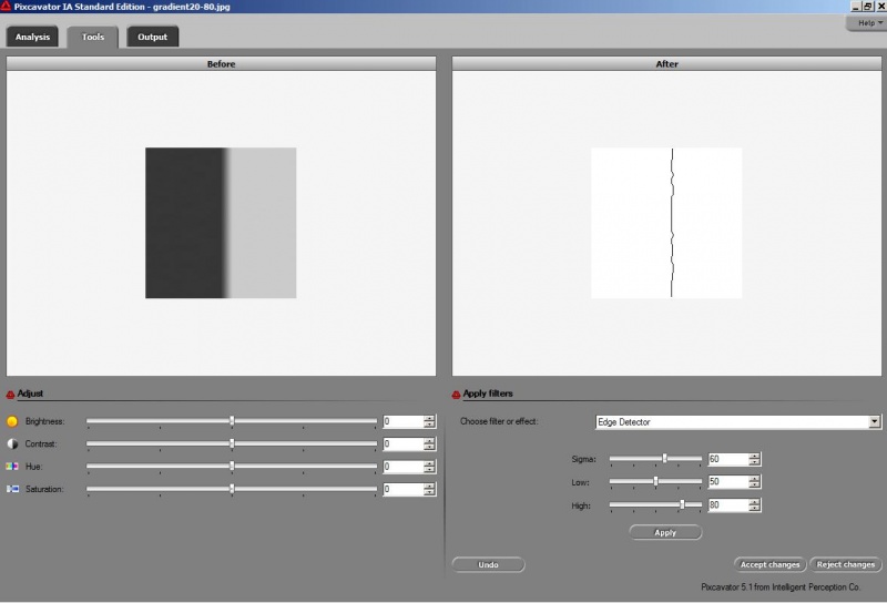
Mathematically, we deal with

 the rate of change of the gray level

             = the gradient of the gray scale function.

(In fact, one only needs the norm of the gradient.) Computation of the derivative however in the digital (discrete) context is a challenge as it is severely affected by noise. Consider the image of coins and its version with noise added.

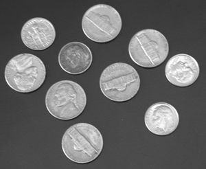
If now edge detection is run, the results are unsatisfactory - too many irrelevant contours. 

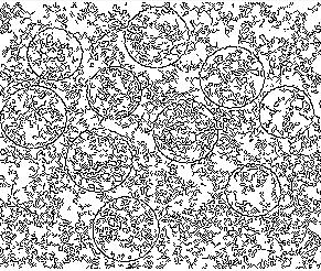
Of course it may be possible to filter out the smaller contours. In this particular case it’s impossible because they are parts of large ones. In fact they form large fractal-like structures. This is the reason why edge detection may have to be preceded by smoothing of the image.

Read more…

Under Review summary (in Output tab) Pixcavator shows the data about the objects found in the image. Pixcavator displays the total area of dark and the total area of light objects – as percentages of the total size of the image (second row).

Under certain circumstances though, the contours of the same kind may be “nested” and, as a results, these percentages may be wrong or even above 100%.

Example below (measuring grass coverage): the dark shows the 151% coverage.

The number is certainly meaningless (there will be a warning about that in the next release).

Why is it above 100%? Because the area is covered several times by these objects. If you click “Color objects”, you’ll see one large object with red contour and many others inside of it.

What happens is easier to see in this simpler image:

The results of image analysis may considered “good” here, but only in the sense that we have captured some 3D information. In general, we restrict our attention to image with mostly 2d information (see Images appropriate for analysis).

What exactly happens here? The way Pixcavator’s sliders operate is this: the contour is allowed to grow until its size (or contrast) is over the bound set by the corresponding slider. Practically, this means that each potential contour C is compared to a contour C’ corresponding to the previous gray level. Then, if C passes but C’ does not then C is plotted.

For more, see Nested boundaries.

In the last post I discussed some issues you encounter when you want to evaluate vegetation coverage based on image analysis.

Now, the area covered should be just a step towards what we are really interested in - the height of the vegetation (or volume, even better).

Let’s consider how one can compute the height of vegetation from a digital image. The idea is very simple:

 the average height = the area / the width.

Consider now what we see in the image.

Views from a side (vegetation in green) and from above:

Assumptions:

1. The board is a square and its dimensions are known.
2. The board is vertical (otherwise it’s impossible to know where the bottom is).
3. The bottom of the board is horizontal on the horizontal (along the board) ground.
4. The field of view of the camera includes the edge of the vegetation and the top of the board.

Then, the average height computed as below is independent from:

• the deviation of the angle of the camera from the horizontal,
• the distance from the camera to the board,
• the height of the position of the camera above the ground.

The measurements (the image in black, the bottom of the board in red):

These come from image analysis:

 A = the area of the board visible above the vegetation (sq pixel),
 W = the width of the board (pixel).

This is known:

 S = the length of the side of the board (in).

Then average height of the vegetation above the ground (in) is:

  H = S * (1 - A / W2).

Computations here.