Computer Vision & Math contains: mathematics courses, covers: image analysis and data analysis, provides: image analysis software. Created and run by Peter Saveliev.

From Computer Vision and Math

Previously we developed a general approach to topological analysis of Binary Images. However, images are rarely binary in computer vision applications.

What we are trying to find in the image

Before we start to develop the algorithm for analysis of gray scale images, let’s first figure out what we are looking for.

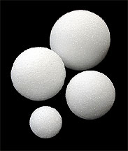
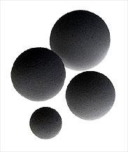
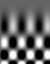
We want to find objects in the image. It seems clear that there are 4 light objects on the dark background in the image on the left. Its negative on the right has 4 dark objects on the light background. Now we need to teach the computer see what we see.

The image:

Its blurry version:

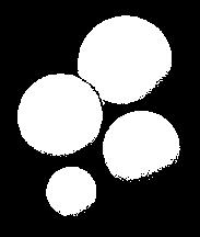
So, what are those "objects"? The idea comes from considering binary images. Indeed, objects in a binary image are either clusters of adjacent black pixels surrounded by white background, or clusters of adjacent white pixels surrounded by black background, like the one on the right.

Therefore, objects in a gray scale image should be either connected darker regions surrounded by lighter background, or connected lighter regions surrounded by darker background. On the pixel level this is what we see:

4 black objects, one with a hole:

3 dark objects, one with a hole:

To confirm that this approach makes sense in real life, see these examples of image analysis or simply run Pixcavator.

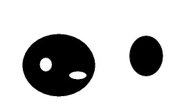
Two dark objects each with a hole:

For more on this see Objects in gray scale images.

Objects as maxima and minima of the gray scale function

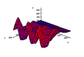
The level of gray of each pixel is given by a number between 0 and 255. These numbers together form the gray scale function of the image. An example is on the right.

A grayscale image:

The gray scale function of the image on the left:

The image on the left is accompanied by its gray scale function. Higher means lighter and lower means darker.

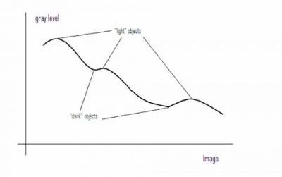
The objects in the image correspond to maxima and minima of the gray scale function. This way, as before, they are either connected darker regions surrounded by lighter background, or connected lighter regions surrounded by darker background. Just like with binary images we have to choose one of these two options. Once again we choose the former.

Grayscale images are treated as if they have dark objects on light background.

Here, the image has 12 dark and 8 light objects. Keep in mind that since the light objects are holes, the ones that touch the border are not counted.

The gray level function of the original image:

The three light objects contained in the image:

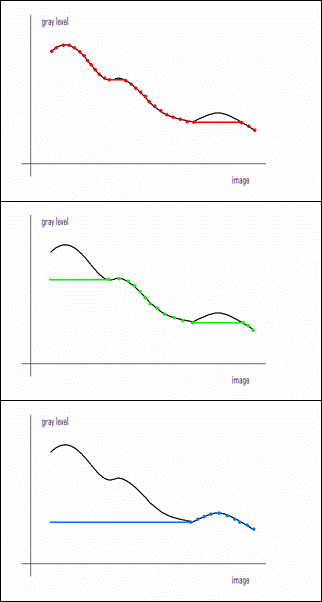
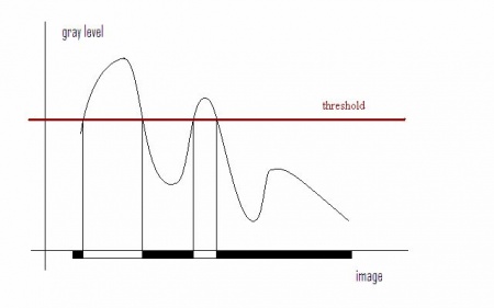
The way we capture light objects may be described as “cutting off mountaintops”, as shown here. On the left, we have the gray level function of the (1-dimensional) image. The maxima and minima are clearly identified as objects. Now, to extract a given dark object as a separate gray scale image, cut off all other maxima.

Similarly, we capture dark objects by "filling in valleys" or removing all other minima.

A gray scale image and its two objects represented as gray scale images:

For more, see Gray scale function.

Thresholding

Our objective is to extend the method described in Binary images to gray scale images. Recall our approach:

In this case the combination will be a sequence. For a given gray scale image we will create a sequence of binary images which we will call frames. Each frame is obtained through thresholding, as follows:

Given a number, threshold, T between 0 and 255, 
create a $T$-th frame by replacing all the pixels 
with gray level lower than or equal to T with black (0), 
the rest with white (1).

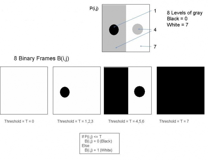
For example, the pixel with gray level of 100 will be white in the first 101 binary images in the sequence and black in the rest. The procedure is illustrated in the picture below. Now, if we let T run from 0 to 255, we end up with a sequence of 256 binary images.

The diagram below illustrates the thresholding procedure and creation of frames. The original gray scale image is at the top. It has 8 levels of gray. Thresholding produces only 4 binary frames because some intermediate levels of gray do not appear in the image. Here P(i,j) stands for the value of the pixel $(i,j)$ in the original, while $B(i,j)$ is the value of that pixel in the binary frame.

For more details see Thresholding.

Counting objects in the sequence of frames

Once the frames have been created, each of them can be - separately - analyzed by the algorithm from Binary images. For example, in the sequence above the algorithm will produce the following: 0, 1, 2, and 1 objects respectively. The total count of 4 would of course be wrong as the number of objects in the gray scale image which is 2. The key is, therefore, not to over-count objects as you move from frame to frame.

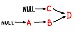
To ensure the correct count, the following rule may be applied: Don't count an object that has a predecessor in the previous frame. Then only A and C should be counted below.

The following, equivalent, rule will prove itself more convenient:

In other words, we count objects that merge with others in the next frame. According to this rule only B and C should be counted.

Note: The last frame is always all black. So, this object is never counted unless it's the only object. Sometimes, the last frame, or any all black frame, and the first frame, or any all white frame, will be simply ignored.

These relations are easier to visualize with a graph, below. The merge of B and C is clearly shown.

We will call this the topology graph. Transition from frame to frame involves Adding Pixels. As a result, each arrow in this graph hides multiple intermediate steps.

For more, see Topology graph.

See next Pseudocode for gray scale images or Algorithm for Grayscale Images.

Using cycles to capture objects

Both objects and holes are captured by cycles. Until later, by cycles we will understand circular sequences of edges. There are 0- and 1-cycles:

• 0-cycles represent objects or connected components of the image,
• 1-cycles represent holes.

This results in a natural and unambiguous representation of the regions by the curves that enclose them. A 0-cycle is traversed clockwise (on the outside of the object like a rubber band) and a 1-cycle is traversed counterclockwise. Observe that in the either case black is on the left.

The binary image. Topological analysis: Two components, the first one with two holes:

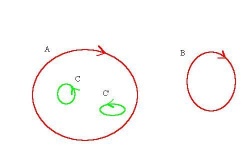
The topological features are captured by cycles. Here A and B are 0-cycles, C and C’ are 1-cycles (outside components clockwise and inside holes counterclockwise):

The analysis should be similar for gray scale images, in spite of the blur. There should be cycles capturing components and holes. The only difference is that there will be more then one possible answer.

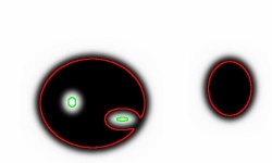
The blurred version of the above binary. A possible topological analysis: Two components, the first one with two holes:

The topological features are captured by cycles. The result does not have to match that of the binary image:

The result of this topological analysis is a partition of the image. A partition is a collection of non-overlapping regions, connected sets of black pixels and connected sets of white pixels, that covers the whole image. The partition is achieved by finding boundaries of these regions as 0- and 1-cycles. These cycles are closed curves made of vertical and horizontal edges of pixels.

The output

The primary output of the algorithm will be the full graph of the frame sequence with framed nodes identified. Based on this information, the topology graph can be extracted. It captures the complete information about the internal structure of the image sequence, including the hierarchy of objects. It is fair, therefore, to call the method lossless, as before.

During processing of each frame, the areas, perimeters, etc of the objects are computed as before, see Binary Images#The output of the algorithm . The algorithm also evaluates certain new characteristics. The main are contrast and "saliency".

By contrast we understand the difference of the gray level of the object and that of the area surrounding the object from the outside measured in levels of gray. The possible levels run from 0 to 255. The lowest setting always produces a copy of the original image, the highest a blank image.

Saliency is what we decided to call the volume under the graph of the function that represents the gray scale image. It is computed by adding the (binary) areas in consecutive frames. Based on that the gray scale centroids are also computed. A direct way to compute them is here [1], in MATLAB.

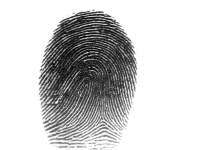
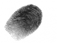
The distribution of these parameters also serves as output. This output can be used in image recognition and image-to-image search. This is why it is important that the count of objects is not significantly affected by rotations. The output for the original 640×480 fingerprint in this image is 3121 dark and 1635 light objects. For the rotated version, it is 2969-1617. By considering only objects with area above 50 pixels, the match becomes better: 265-125 and 259-124, respectively.

Stretching the image does not affect the number of objects. The distribution of objects with respect to area is affected but in an entirely predictable way. Shrinking makes objects merge. If the goal, however, is to count and analyze large features, limited shrinking of the image does not affect the outcome. The counting is also stable under “salt-and-pepper” noise or mild blurring. Our experience has shown that the output corresponds well with what humans see. The only case when there is a mismatch is when the size, or the contrast of the object, or its connection to another object are imperceptible to the human eye.

Indirectly, cycles as sequences of edges are captured. This data can be used as follows. (1) The cycles can be plotted in black to reveal boundaries of a gray-scale image. This creates a black-and-white “drawing”, below. (2) If they are filled with an appropriate choice of colors, the user can view a new, simplified, image. (3) The interior of the cycles can be recolored randomly to exhibit them. (4) The cycles can be used for further, possibly manual, editing by the user. For example, they can be moved around or deformed. (5) Besides visualization, the boundaries can be extracted and used elsewhere. For example, they can be matched with cycles collected from another image, or used for picture enlargement, or separation of foreground from background.

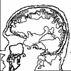
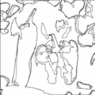
Example of the output: the first is the original image and the second is some of its cycles.

Consider also Image Simplification.

To experiment with the concepts, download the free Pixcavator Student Edition.