Robustness of topology of digital images and point clouds by Saveliev

Robustness of topology of digital images and point clouds by Peter Saveliev

Abstract. Such modern applications of topology as digital image analysis and data analysis have to deal with noise and other uncertainty. In this environment, the data structures often appear "filtered" into a sequence of cell complexes. We introduce the homology group of the filtration as the group of all possible homology classes of all elements of the filtration without double count. The second step of analysis is to discard the features that lie outside the user's choice of the acceptable level of noise.

1 1. Introduction

Since Poincare, homology has been used as the main descriptor of the topology of geometric objects. In the classical context, however, all homology classes receive equal attention. Meanwhile, applications of topology in analysis of images and data have to deal with noise and other uncertainty. This uncertainty appears usually in the form of a real valued function defined on the topological space. Persistence is a measure of robustness of the homology classes of the lower level sets of this function \ELZ, \Carlsson, \CZ09, \CZ.

Since it's unknown beforehand what is or is not noise in the dataset, we need to capture all homology classes including those that may be deemed noise later. In this paper we introduce an algebraic structure that contains, without duplication, all these classes. Each of them is associated with its persistence and can be removed when the acceptable threshold for noise is set. The last step can be carried out repeatedly in order to find the best possible threshold. The approach follows the approach to analysis of digital images presented in \Sav1.

2 2. Background

The topological spaces subject to such analysis are cell complexes. A cell complex is a combinatorial structure that describes how $k$-dimensional cells are attached to each other along $(k-1)$-dimensional cells. Cell complexes come from the following two main sources.

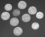
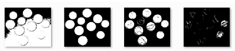
First, a gray scale image is a real-valued function $f$ defined on a rectangle. Given a threshold $r$, the lower level set $f^{-1}((-\infty ,r))$ can be thought of as a binary image. Each black pixel of this image is treated as a square cell in the plane. These 2-dimensional cells are combined with their edges (1-cells) and vertices (0-cells) and in the $n$-dimensional case, the image is decomposed into a combination of $0$-, $1$-,..., $n$-cubes. This process is called thresholding. The result is a cell complex $K$ for each $r,$ see \KMM.

--> -->

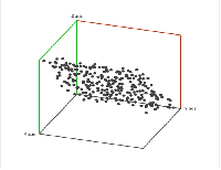
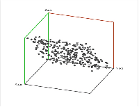
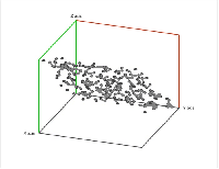
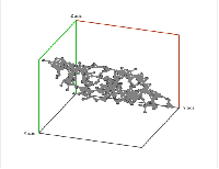
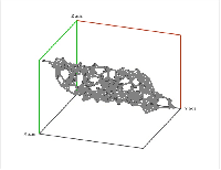
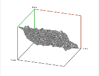
Second, a point cloud is a finite set $S$ in some Euclidean space of dimension $d$. Given a threshold $r$, we deem any two points that lie within $r$ from each other as "close". In this case, this pair of points is connected by an edge. Further, if three points are "close", pairwise, to each other, we add a face spanned by these points. If there are four, we add a tetrahedron, and, finally, any $d+1$ "close" points create a $d$-cell. The process is called the Vietoris-Rips construction. The result is a cell complex $K$ for each $r$ \ELZ.

-->

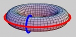
Next, we would like to quantify the topology of the cell complex $K.$ It is done via the Betti numbers of $K$: $B_{0}$ is the number of connected components in $K$; $B_{1}$ is the number of holes or tunnels (1 for letter O or the donut; 2 for letter B and the torus); $B_{2}$ is the number of voids or cavities (1 for both the sphere and the torus), etc.

The Betti numbers are computed via homology theory \Bredon. One starts by considering the collection $C_{k}(K)$ of all formal linear combinations (over a ring $R$) of $k-$cells in $K,$ called chains.

Combined they form a finitely generated abelian group called the chain complex $C_{k}(K)$, or collectively $C_{\ast }(K).$ A $k$-chain can be recorded as an $N_{k}$-vector, where $N_{k}$ is the total number of $k$-cells in $K$. The boundary of a $k$-chain is the chain comprised of all $(k-1)$-faces of its cells taken with appropriate signs. Then the boundary operator $\partial :C_{k}(K)\rightarrow C_{k-1}(K) $ acts on the chain complex and is represented by a $N_{k}\times N_{k-1}$ matrix.

From the chain complex $C_{\ast }(K),$ the homology group is constructed by means of the standard algebraic tools. To capture the topological features one concentrates on cycles, i.e., chains with zero boundary, $ \partial A=0$.

Further, one can verify whether two given $k$-cycles $A$ and $B$ are homologous: the difference between them is the boundary of a $(k+1)$-chain $T:A-B=\partial T$ (such as two meridians of the torus). In this case, $A$ and $B$ belong to the same homology class $H=[A]=[B]$.

The totality of these equivalence classes in each dimension $k$ is called the $k$-th homology group $H_{k}(K)$ of $K$, collectively $H_{\ast }(K)$. Then, Betti number $B_{k}$ is the rank of $H_{k}(K)$.

3 3. Prior work and outline

The methods for computing homology groups are well developed. In real-life applications however both digital images and point clouds may be noisy and one needs to evaluate the significance of their homology classes. The approach to this problem has been the following. Instead of using a single threshold and studying a single cell complex, one considers all thresholds and all possible cell complexes.

Since increasing threshold $r$ enlarges the corresponding complex, we have a sequence of complexes: \begin{equation*} K^{1}\hookrightarrow K^{2}\hookrightarrow K^{3}\hookrightarrow K^{4}\hookrightarrow \ldots \ \hookrightarrow K^{s}, \end{equation*} where the arrows represent the inclusions: $i^{n,n+1}:K^{n}\hookrightarrow K^{n+1}.$ Let $i^{nm}:K^{n}\hookrightarrow K^{m},n\leq m,$ also be the inclusion. This structure $\{K^{n},i^{nm}\}$ is called a filtration.

Now, each of these inclusions generates a homomorphism $i_{\ast }^{nm}:H_{\ast }(K^{n})\rightarrow H_{\ast }(K^{m})$ called the homology map induced by }$i^{nm}.$ As a result, we have a sequence of homology groups connected by these homomorphisms: \begin{equation*} H_{\ast }(K^{1})\rightarrow H_{\ast }(K^{2})\rightarrow \ldots \ \rightarrow H_{\ast }(K^{s})\longrightarrow 0. \end{equation*} These homomorphisms record how the homology changes as the complex grows at each step. For example, a component appears and then merges with another one, or a hole is formed and then filled. We refer to these events as birth and death of the corresponding homology classes.

In order to evaluate the robustness of an element of one of these groups the persistence of a homology class is defined as the number of steps it takes for the class to end at $0.$ In other words, \begin{equation*} \text{persistence = death date - birth date.} \end{equation*} The $p$-persistent homology group of $K^{i}$ is defined as the image of $i_{\ast }^{i,i+p}.$ It's what's left from $H_{\ast }(K^{i})$ after $p$ steps in the filtration. Now the robustness of the homology classes of the filtration is evaluated in terms of the set of intervals $[birth,death]$ representing the life-spans, called barcodes, of the homology classes \CZ.

Our approach is somewhat different. It consists of two steps.

First step: we pool all possible homology classes in all elements of the filtration together in a single algebraic structure (Sections 4 and 5). The presence of noise is ignored. The homology group $H_{\ast }(\{K^{n}\})$ of filtration $\{K^{n}\}$ captures all homology classes in the whole filtration -- without double counting.

Second step: for a given positive integer $p,$ the $p$-noise group $N_{\ast }^{p}(\{K^{n}\})$ is comprised of the homology classes in $H_{\ast }(\{K^{n}\})$ with the persistence less than $p.$ Next, we "remove" the noise from the homology group of filtration by using the quotient (Sections 6 and 7): \begin{equation*} H_{\ast }^{p}(\{K^{n}\})=H_{\ast }(\{K^{n}\})/N_{\ast }^{p}(\{K^{n}\}). \end{equation*} In other words: if the difference between two homology classes is deemed noise, they are equivalent. The second step can be repeated as needed.

We also discuss the computational aspects of this approach (Section 8) and multiparameter filtrations (Section 9).

Our approach provides a coarser classification of the homology of filtrations than the one based on barcodes. The reason is that all homology classes with long enough life-spans, i.e., high persistence, have equal place in the homology group $H_{\ast }(\{K^{n}\})$ of the filtration regardless of the time of birth and death.

4 4. Motivation: the homology of a gray scale image

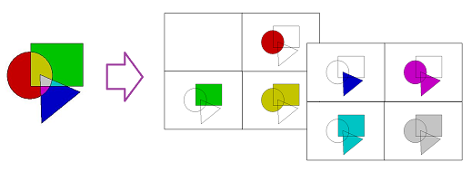
In this section we will try to understand the meaning of the homology of the gray scale image in Figure 1 below. For simplicity we assume that there are only 2 levels of gray in addition to black and white. A visual inspection of the image suggests that it has three connected components each with a hole. Therefore, its $0$- and $1$-homology groups should have three generators each. We now develop an algebraic procedure to arrive at this result.

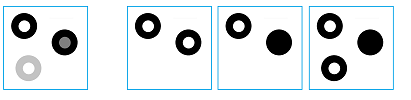
First the image is "thresholded". The lower level sets of the gray scale function of the image form a filtration: a sequence of three binary images, i.e., cell complexes: $K^{1}\hookrightarrow K^{2}\hookrightarrow K^{3},$ where the arrows represent the inclusions. Suppose $A_{i},B_{i},C_{i}$ are the homology classes that represent the components of $K^{i}$ and $% a_{i},b_{i},c_{i}$ are the holes, clockwise starting at the upper left corner. The homology groups of these images also form sequences -- one for each dimension 0 and 1.

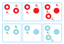
Suppose $F_{1},F_{2}$ are the two homology maps, i.e., homomorphisms of the homology groups generated by the inclusions of the complexes, with $F_{3}=0$ included for convenience. These homomorphisms act on the generators, as follows: \begin{eqnarray*} A_{1} &\rightarrow &A_{2}\rightarrow A_{3}\rightarrow 0,B_{1}\rightarrow B_{2}\rightarrow B_{3}\rightarrow 0, \\ C_{2} &\rightarrow &C_{3}\rightarrow 0,a_{1}\rightarrow a_{2}\rightarrow a_{3}\rightarrow 0, \\ b_{1} &\rightarrow &0,c_{3}\rightarrow 0. \end{eqnarray*}

To avoid double counting, we want to count only the homology classes that don't reappear in the next homology group. As it turns out, a more algebraically convenient way to accomplish this is to count only the homology classes that go to $0$ under these homomorphisms. These classes form the kernels of $F_{1},F_{2},F_{3}$. Now, we choose the homology group of the original, gray scale image to be the direct sum of these kernels: \begin{equation*} H_{0}(\{K^{i}\})=<A_{3},B_{3},C_{3}>,\text{ }H_{1}(\{K^{i}% \})=<b_{1},a_{3},c_{3}>. \end{equation*} Thus the image has three components and three holes, as expected.

5 5. Homology groups of filtrations

In the following sections we provide formal definitions. All cell complexes are finite.

Suppose we have a one-parameter filtration: \begin{equation*} K^{1}\hookrightarrow K^{2}\hookrightarrow K^{3}\hookrightarrow \ldots \ \hookrightarrow K^{s}. \end{equation*} Here $K^{1},K^{2},\ldots ,K^{s}$ are cell complexes and the arrows represent the inclusions $i^{n,n+1}:K^{n}\hookrightarrow K^{n+1}$ and so do $% i^{nm}:K^{n}\hookrightarrow K^{m},n\leq m$. We will denote the filtration by $\{K^{n},i^{nm}:n,m=1,2,...,s,n\leq m\},$ or simply $\{K^{n}\}.$ Next, homology generates a "direct system" of groups and homomorphisms: \begin{equation*} H_{\ast }(K^{1})\rightarrow H_{\ast }(K^{2})\rightarrow \ldots \ \rightarrow H_{\ast }(K^{s})\longrightarrow 0. \end{equation*} We denote this direct system by $\{H_{\ast }(K^{n}),i_{\ast }^{nm}:n,m=1,2,...,s,n\leq m\},$ or simply $\{H_{\ast }(K^{n})\}.$ The zero is added in the end for convenience.

Our goal is to define a single structure that captures all homology classes in the whole filtration without double counting. The rationale is that if $x\in H_{\ast }(K^{n}),y\in H_{\ast }(K^{m}),$ $y=i_{\ast }^{nm}(x),$ and there is no other $x$ satisfying this condition, then $x$ and $y$ may be thought of as representing the same homology class of the geometric object behind the filtration.

The homology group of filtration $\{K^{n}\}$ is defined as the product of the kernels of the inclusions: \begin{equation*} H_{\ast }(\{K^{n}\})=\ker i_{\ast }^{1,2}\oplus \ker \,i_{\ast }^{2,3}\oplus \ldots \oplus \ker i_{\ast }^{s,s+1}. \end{equation*} Here, from each group we take only the elements that are about to die. Since each dies only once, there is no double-counting. Since the sequence ends with $0,$ we know that everyone will die eventually. Hence every homology class appears once and only once.

These are a few simple facts about this group.

Proposition. If $i_{\ast}^{n,n+1}$ is an isomorphism for each $n=1,2,...,s-1,$ then $H_{\ast}(\{K^{n}\})=H_{\ast}(K^{1})$ $.$

Proposition. If $i_{\ast}^{n,n+1}$ is a monomorphism for each $n=1,2,...,s-1,$ then $H_{\ast}(\{K^{n}\})=H_{\ast}(K^{s}).$

Proposition. Suppose $\{K^{n},i^{nm},n,m=1,2,...,s\}$ and $\{L^{n},j^{nm},n,m=1,2,...,s\}$ are filtrations. Then $H_{\ast}(\{K^{n}\sqcup L^{n}\})=H_{\ast}(\{K^{n} \})\oplus H_{\ast}(\{L^{n}\}).$

Proposition. Suppose $\{K^{n},i^{nm},n,m=1,2,...,s\}$ and $\{L^{n},j^{nm},n,m=1,2,...,s\}$ are filtrations and $f:K^{s}\rightarrow L^{s}$ is a cell map. Then the homology map of the homology groups of these filtrations $f_{\ast}:H_{\ast }(\{K^{n}\})\rightarrow H_{\ast}(\{L^{n}\})$ is well defined as \[ f_{\ast}(x_{1},x_{2},...,x_{s})=(f_{\ast}^{1}(x_{1}),f_{\ast}^{2}% (x_{2}),...,f_{\ast}^{s}(x_{s})), \] where $f^{n}$ is the restriction of $f$ to $K^{n}.$

The stability of the homology group of a filtration follows from the stability of its persistence diagram, i.e., the set of points $\{(birth,death)\}\subset \mathbf{R}^{2}$ for the generators of the homology groups of the filtration, plus the diagonal. It is proven in \CEH that $d_{B}(D(f),D(g))\leq ||f-g||_{\infty },$ where $d_{B}$ is the bottle-neck distance between the persistence diagrams $D(f),D(g)$ of two filtrations generated by tame functions $f,g.$ Function $F(x,y)=y-x$ creates an analogue bottle-neck distance for the set of points $\{persistence\}\subset \mathbf{R} $ and its stability follows from the continuity of $F$.

6 6. Motivation: the high contrast homology of a gray scale image

To justify our approach to persistence, we observe that some of the features in the image in Figure 1 are more prominent than others. In particular, some of the features have lower contrast. These are the holes in the second and the third rings as well as the third ring itself. By contrast of a lower level set of the gray level function we understand the difference between the highest gray level adjacent to the set and the lowest gray level within the set.

An easy computation shows that the homology classes with persistence of 3 or higher among the generators are: $A_{1},B_{1},a_{1}.$ However, the set of the classes of high persistence isn't a subgroup of the homology group of the respective complex. Instead, we look at the classes with low persistence, i.e., the noise. In particular, the classes in $H_{\ast }(K^{1})$ of persistence 2 or lower form the kernel of $F_{2}F_{1}$. We now "remove" this noise from the homology groups of the filtration by considering their quotients over these kernels. In particular, the 3-persistent homology groups of the image are: \begin{align*} H_{0}^{3}(\{K^{i}\})& =<A_{1},B_{1}>/0=<A_{1},B_{1}>, \\ H_{1}^{3}(\{K^{i}\})& =<a_{1},b_{1}>/<b_{1}>=<a_{1}>. \end{align*} Observe that the output is identical to the homology of a single complex, i.e., a binary image, with two components and one hole. The way persistence is defined ensures that we can never remove a component as noise but keep a hole in it.

Observe now that the holes in the second and third rings have the same persistence (contrast) and, therefore, occupy the same position in the homology group regardless of their birth dates (gray level). Second, if we shrunk one of these rings, its persistence and, therefore, its place in the homology group wouldn't change. These observations confirm the fact that the homology group of the gray scale image, unlike the barcodes, captures only its topology.

In the case of a Vietoris-Rips complex, not only the barcode, the interval $[birth, death]$, but also the persistence, the number $death - birth$, of a homology class contains information about the size of representatives of these classes. For example, a set of points arranged in a circle will produce a $1$-cycle with twice as large birth, death, and persistence than the same set shrunk by a factor of 2. However, persistence defined as $death/birth$ will have the desired property of scale independence. The same result can be achieved by an appropriate re-parametrizing of the filtration.

7 7. Persistent homology groups of filtrations

In the general context of filtrations the measure of importance of a homology class is its persistence which is the length of its lifespan within the direct system of homology of the filtration.

Given filtration $\{K^{n}\},$ we say that the persistence $P(x)$ of $x\in H_{\ast}(K^{n})$ is equal to $p$ if $i_{\ast }^{n,n+p}(x)=0$ and $i_{\ast}^{n,n+p-1}(x)\neq0.$ Our interest is in the "robust" homology classes, i.e., the ones with high persistence. However, the collection of these classes is not a group as it doesn't even contain 0. So we deal with "noise" first. Given a positive integer $p,$ the $p$-noise (homology) group $N_{\ast}^{p}(K^{n})$ of $\{K^{n}\}$ is the group of all elements of $K^{n}$ with persistence less than $p.$

Alternatively, we can define these groups via kernels of the homomorphisms of the inclusions: $N_{\ast }^{p}(K^{n})=\ker \,i_{\ast }^{n,n+p}.$

Proposition. $N_{\ast}^{p+1}(K^{n})\subset N_{\ast}^{p}(K^{n}).$

Next, we "remove" the noise from the homology group. The $p$-persistent (homology) group} of $K^{n}$ with respect to the filtration $ \{K^{n}\}$ is defined as \begin{equation*} H_{\ast }^{p}(K^{n})=H_{\ast }(K^{n})/N_{\ast }^{p}(K^{n}). \end{equation*} The point of this definition is that, given a threshold for noise, if the difference between two homology classes is noise, they should be equivalent.

Next, just as in the case of noise-less analysis, we define a single structure to capture all (robust) homology classes. Let $p$ be a positive integer. Suppose $x\in \ker i_{\ast }^{k,k+p}$ and let $y=$ $i_{\ast }^{k,k+1}(x).$ Then \begin{eqnarray*} i_{\ast }^{k+1,k+1+p}(y) &=&i_{\ast }^{k+1,k+1+p}(i_{\ast }^{k,k+1}(x)) \\ &=&i_{\ast }^{k,k+1+p}(x)=i_{\ast }^{k+p,k+p+1}(i_{\ast }^{k,k+p}(x)) \\ &=&i_{\ast }^{k+p,k+p+1}(0)=0. \end{eqnarray*} Hence $y\in \ker i_{\ast }^{k+1,k+1+p}.$ We have proved that \begin{equation*} i_{\ast }^{k,k+1}(\ker i_{\ast }^{k,k+p})\subset \ker i_{\ast }^{k+1,k+1+p}. \end{equation*} It follows that the homomorphism $i_{\ast }^{k,k+1}:\ker i_{\ast }^{k,k+p}\rightarrow \ker i_{\ast }^{k+1,k+1+p}$ generated by the inclusion is well-defined.

Next, we use these homomorphisms to define the $p$-noise (homology) group $N_{\ast }^{p}(\{K^{n}\})$ of filtration $\{K^{n}\}$ as \begin{equation*} N_{\ast }^{p}(\{K^{n}\})=\ker i_{\ast }^{1,2}\oplus \ldots \oplus \ker i_{\ast }^{s,s+1}. \end{equation*} Observe that the formula is the same as the one in the definition of $H_{\ast }^{p}(\{K^{n}\}).$ Since $i_{\ast }^{k,k+1}:\ker i_{\ast }^{k,k+p}\rightarrow \ker i_{\ast }^{k+1,k+1+p}$ is a restriction of $ i_{\ast }^{k,k+1}:H_{\ast }^{p}(K^{k})\rightarrow H_{\ast }^{p}(K^{k+1}),$ each term in the above definition is a subgroup of the corresponding term in the definition of $H_{\ast }(\{K^{n}\}).$ The proposition below follows.

Proposition. $N_{\ast }^{p}(\{K^{n}\})\subset H_{\ast }(\{K^{n}\}).$

Finally, the $p$-persistent (homology) group of filtration $\{K^{n}\}$ is \begin{equation*} H_{\ast }^{p}(\{K^{n}\})=H_{\ast }(\{K^{n}\})/N_{\ast }^{p}(\{K^{n}\}). \end{equation*}

The results about $H_{\ast }^{p}(\{K^{n}\})$ analogous to the ones about $H_{\ast }(\{K^{n}\})$ in Section 5 hold.

8 8. Computational aspects

For 2-dimensional gray scale images, this approach to homology and persistence has been used in an image analysis program called Pixcavator.

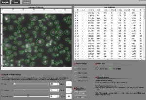
The algorithm described in \Sav1 has complexity of $O(n^{2}),$ where $n$ is the number of pixels in the image.

For the general case, the analysis algorithm may be outlined as follows:

• The input is a filtration.
• The homology groups of its members and the homomorphisms induced by inclusions are computed.
• The homology group of the filtration is computed.
• The persistence of all elements of the homology groups is computed.
• The user sets a threshold $p$ for persistence and the $p$-noise group of the filtration is computed.
• The $p$-persistent homology group of the filtration is computed and given as output.

If the user changes the threshold, the last step is repeated as necessary without repeating the rest.

The algorithm above computes the homology group of filtration, as defined, incrementally. This may be both a disadvantage and an advantage. In comparison, the persistence complex \CZ also contains information about all homology classes of the filtration but its computation does not require computing the homology of each complex of the filtration. Meanwhile, the above algorithm may have to compute the same homology over and over if consecutive complexes are identical. Hence, the algorithm has a disadvantage in terms of processing time. On the other hand, the incremental nature of the algorithm makes its use of memory independent from the length of the filtration. Another advantage is that multi-parameter filtrations are dealt with in the exact same manner (see next section).

The inefficiency of the above algorithm can be addressed with a proper algebraic tool. This tool is the mapping cone \Weibel.

Suppose, for simplicity, that our filtration has only two elements: $i:K^{1} \hookrightarrow K^{2}.$ The mapping cone is, in a sense, a combination of the kernel and the cokernel of $i_{\ast }$. It captures the difference between $K^{1}$ and $K^{2}$ on the chain level: everything in $C_{\ast }(K^{1})$ is killed unless it also appears in $C_{\ast }(K^{2})$ under $% i_{\ast }$. Then the algorithm is to construct the homology group from the chain complexes $C_{\ast }(K^{1}),C_{\ast }(K^{2})$ of the elements of the filtration and the chain map $i_{\ast }:C_{\ast }(K^{1})\rightarrow C_{\ast }(K^{2}).$

9 9. Multiparameter filtrations

Multiparameter filtrations come from the same main sources as one-parameter filtrations.

First, color images are thresholded according to their three color channels.

Second, point clouds are "thresholded" by the closeness of their points and, for example, the density of the points.

Let's limit our attention to the two-parameter case. A (finite) two-parameter filtrations $\{K^{nm}\}$ is a table of complexes connected by inclusions \begin{equation*} i(n,m,n+p,m+q):K^{nm}\rightarrow K^{n+p,m+q},p,q\geq 0, \end{equation*} These inclusions generate homomorphisms \begin{equation*} i_{\ast }(n,m,n+q,m+p):H_{\ast }(K^{nm})\rightarrow H_{\ast }(K^{n+q,m+p}), \end{equation*} with 0s added in the end of each row and each column. Define the homology group of the filtration $\{K^{nm}\}$ as \begin{eqnarray*} H_{\ast }(\{K^{nm}\}) = {\displaystyle\bigoplus\limits_{n}}\ker i_{\ast }(n,m,n+1,m)\cap \ker i_{\ast }(n,m,n,m+1). \end{eqnarray*} The analogues of the results in Section 5 hold.

There are many ways to define persistence in the multiparameter setting. For example, we can evaluate the robustness of a homology class $x\in H_{\ast }(K^{nm})$ in terms of the pairs $(p,q)$ of positive integers satisfying \begin{equation*} i_{\ast }(n,m,n+p,m)(x)=0\text{ and }i_{\ast }(n,m,n,m+q)(x)=0. \end{equation*} Next, just as in Section 7, we restrict the homomorphisms generated by the inclusions to the homology classes of low persistence: \begin{eqnarray*} i_{\ast }(n,m,n+1,m) &:& \\ \ker i_{\ast }(n,m,n+p,m) &\rightarrow &\ker i_{\ast }(n+1,m,n+1+p,m), \\ i_{\ast }(n,m,n,m+1) &:& \\ \ker i_{\ast }(n,m,n,m+q) &\rightarrow &\ker i_{\ast }(n+1,m,n,m+1+q). \end{eqnarray*} Then the $(p,q)$-noise group of $K^{nm}$ is defined via these homomorphisms: \begin{eqnarray*} N_{\ast }^{pq}(\{K^{nm}\}) = {\displaystyle\bigoplus\limits_{n}}\ker i_{\ast }(n,m,n+1,m)\cap \ker i_{\ast }(n,m,n,m+1). \end{eqnarray*} Finally, the $(p,q)$-persistent (homology) group of filtration $\{K^{nm}\}$ is defined as \begin{equation*} H_{\ast }^{pq}(\{K^{n}\})=H_{\ast }(\{K^{nm}\})/N_{\ast }^{pq}(\{K^{nm}\}). \end{equation*}

The results about $H_{\ast }^{pq}(\{K^{nm}\})$ analogous to the ones about $ H_{\ast }^{p}(\{K^{n}\})$ in Section 7 hold.

10 Bibliography

1. \Bredon\ G. Bredon, Topology and Geometry, Springer Verlag, 1993.
2. \Carlsson\ G. Carlsson, Topology and data, Bulletin of the Amer. Math. Soc., Vol. 46, No. 2, pp. 255-308, 2010.
3. \CZ\ G. Carlsson and A. Zamorodian, Computing persistent homology. Discrete and Computational Geometry, 2005, 20th ACM Symposium on Computational Geometry, Brooklyn, NY, 2004.
4. \CZ09\ G. Carlsson and A. Zamorodian, The theory of multidimensional persistence. 23rd ACM Symposium on Computational Geometry, Gyeongju, South Korea, 2007. Discrete and Computational Geometry, 2009.
5. \CEH\ D. Cohen-Steiner, H. Edelsbrunner, J. Harer, Stability of persistence diagrams, Discrete and Computational Geometry, vol. 37, no. 1, \ pp. 103-120 (2007).
6. \ELZ\ H. Edelsbrunner, D. Letscher, and A. Zomorodian, Topological persistence and simplification. Discrete Comput. Geom. 28 (2002), pp. 511-533.
7. \KMM\ T. Kaczynski, K. Mischaikow, and M. Mrozek, Computational Homology, Appl. Math. Sci. Vol. 157, Springer Verlag, NY,2004.
8. \Sav1\ P. Saveliev, A graph, non-tree representation of the topology of a gray scale image, Proceedings of SPIE, Algorithms and Systems, 2011, Volume 7870, O1-O19.
9. \Weibel\ C. A. Weibel, An Introduction to Homological Algebra, Cambridge University Press, 1994.