Maps of polyhedra

1 Maps v. cell maps

Previously, we proved that if complex $K^1$ is obtained from complex $K$ via a sequence of elementary collapses, then $$H(K)\cong H(K^1).$$ In spite of its length, the proof was straightforward. However, the result, as important as it is, is a very limited instance of the invariance of homology. We explore next what we can achieve in this area if we take an indirect route and develop a seemingly unrelated theory.

In order to build a complete theory of homology, our long-term goal now is to prove that the homology groups of two homeomorphic, or even homotopy equivalent, spaces are isomorphic -- for the triangulable spaces we call polyhedra.

But these two concepts rely entirely on the general concept of map! Meanwhile, this is the area where our theory remains most inadequate. Even if we are dealing with cell complexes, a map $f:|K|\to |L|$ between their realizations doesn't have to be a cell map. As a result we are unable to define its chain map $f_{\Delta}:C(K)\to C(L)$ and unable to define or compute its homology map $f_*:H(K)\to H(L)$.

The idea of our new approach is to replace a map with a cell map, somehow: $$f:|K|\to |L| \quad\leadsto\quad g:K\to L,$$ and then simply declare that the homology map of the former is that of the latter: $$f_*:=g_*:H(K)\to H(L).$$ But, we have to do this in such a way that this resulting homology map is well-defined. This is a non-trivial task.

Example (self-maps of circle). We have already seen several examples of maps $f:{\bf S}^1 \to {\bf S}^1$ of the circle to itself that aren't cell maps:

Suppose the circle is given by the simplest cell complex with just two cells $A,a$. Let's list all maps that can be represented as cell maps:

• the constant map: $f(u)=A \leadsto g(A)=A',\ g(a)=A$;
• the identity map: $f(u)=u \leadsto g(A) = A',\ g(a) = a'$;
• the flip around the $y$-axis: $f(x,y)=(-x,y) \leadsto g(A)=A',\ g(a) = -a'$.

These are examples of simple maps that aren't cell maps:

• any other constant map;
• any rotation;
• any double-wrapping of the loop (or triple-, etc.);
• the flip around any other axis.

And, we can add to the list anything more complicated than these!

Let's see if we can do anything about this problem.

One approach is to try to refine the given cell complexes. For example, cutting each $1$-cell in half allows us to accommodate a rotation through $180$ degrees:

Indeed, we can set: $$g(A)=g(B):=A',\ g(a):=b',\ g(b):=a'.$$

What about “doubling”? Cutting the only $1$-cell of the domain complex (but not in the target!) in half helps:

Indeed, we can set: $$g(A)=g(B):=A',\ g(a)=g(b):=a'.$$

Can we accommodate the rotation through $180$ degrees by subdividing only the domain? We set: $$g(A)=g(B):=A',\ g(a):=a',\ g(b):=A'.$$ Since $b$ collapses, the representation isn't ideal but it does capture what happens to the $1$-cycle.

$\square$

Exercise. Provide cell map representations of the maps listed above with as few subdivisions as possible.

Exercise. Demonstrate that the rotation of the circle through $\sqrt{2}\pi$ cannot be represented as a cell map no matter how many subdivisions one makes.

2 Cell approximations of maps

There are many more maps that might be hard or impossible to represent as cell maps, such as these maps from the circle to the ring:

If we zoom in on the ring and supply it with a cubical complex structure, we can see that the diagonal lines can't be represented exactly within this grid, no matter how many times we refine it.

The idea is then to approximate these maps:

The meaning of approximation is the same as in other fields: every element of a broad class of functions is substituted -- with some accuracy -- with an element of a narrower, nice class of functions. For example, differential functions are approximated with polynomials (Taylor) or trigonometric polynomials (Fourier). The end-result of such as approximation is a sequence of polynomials converging to the function. This time the goal is

• to approximate continuous functions (maps) with cell maps.

But how do we measure how close two maps are within a complex? Since we want the solution independent from the realization, no actual measurements will be allowed. Instead, we start with the simple idea of using “cell distance” as one and only “measurement” of closedness.

We can say that a cell map $g:K\to L$ approximates a map $f:|K|\to |L|$ at vertex $A$ of $K$ if its value $g(A)$ is within the cell distance from $f(A)$, i.e., there is a cell $\sigma\in L$ such that $$f(A),g(A)\in \sigma. $$

Judging by the above examples, this restriction won't make the functions very close. The only way to allow for cell maps to approximate $f$ better and better and generate a convergent sequence is to refine the complexes. Below we can see how, under multiple subdivisions, cell maps start to get closer to the original:

Even though these approximations seem to work well, they are incomplete as they are defined only on the vertices. We need to extend them to the edges.

We discover that we cannot extend the “cell maps” in 3rd, 5th, and 6th graphs above to $1$-cells. The reason is the same: as $x$ changes by $1$ cell, $y$ changes by $2$ or more.

The idea of how to get around this problem is suggested by the continuity of $f$! Indeed, it will ensure that a small enough increment of $x$ will produce an increment of $y$ as small as we like. Then the plan is to subdivide but subdivide only the domain:

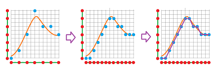
The approach works in the above example, and we will prove that this positive outcome is guaranteed -- after a sufficient number of subdivisions.

Without refining the target space, repeating this approximation doesn't produce a sequence $g_n$ convergent to the original map $f$. For such an approximation to have any value at all, $g_n$ has to become “good enough” for large enough $n$. We will demonstrate that it is good enough topologically: $g_n \simeq f$!

From this point on, we limit ourselves to simplicial and cubical complexes and we refer to them as simply “complexes” and to their elements as “cells”. The reason is that either class has a standard refinement scheme: the barycentric subdivision for simplicial and the “central” subdivision for cubical complexes:

In either case, each cell acquires a new vertex in the middle. For a given complex $k$, the $n$th subdivision of this kind will be denoted by $K^n$ (not to be confused with $K^{(n)}$, which is the $n$th skeleton).

Exercise. Given a cubical complex $K$, list all cells of $K^1$.

In addition to vertices mapped by $f$ and $g$ within a cell from each other, we need to ensure a similar behavior for all other cells. Suppose for a moment that the values of $f$ and $g$ coincide on all vertices of $K$, then any cell $a$ adjacent to a vertex $A$ should be mapped to a cell adjacent to vertex $f(A)=g(A)$. As we recognize a familiar situation, we realize that we are talking about $a$ and $f(a)$ located within the star of the corresponding vertex!

Recall that given a complex $K$ and a vertex $A$ in $K$, the star of $A$ in $K$ is the collection of all cells in $K$ that contain $A$: $${\rm St}_A = {\rm St}_A(K):= \{ \sigma \in K: A\in\sigma\} \subset K,$$ while the open star is the union of the insides of all these cells: $$N_A = N_A(K) = \bigcup\{\dot{\sigma}: \sigma\in St_A(K)\} \subset |K|.$$

We recall also this simple result about simplicial complexes, which also holds for cubical complexes.

Proposition. The set of all open stars of all vertices of complex $K$ forms an open cover of its realization $|K|$.

Exercise. Prove that the set of all open stars of all vertices of all subdivisions of complex $K$ forms a basis of the topology of its realization $|K|$.

We are ready now to state the main definition.

Definition. Suppose $f:|K|\to |L|$ is a map between realizations of two complexes. Then a cell map $g:K\to L$ is called a cell approximation of $f$ if $$f(N_A)\subset N_{g(A)},$$ for any vertex $A$ in $K$.

The condition is illustrated for dimension $1$:

And for dimension $1$:

Observe here that, if we assume again that $f$ and $g$ coincide on the vertices, the above condition is exactly what we have in the definition of continuity: $$f(N_x)\subset N_{f(x)},$$ if $N_x$ stands simply for a neighborhood of point $x$.

Proposition. Cell approximation is preserved under compositions. In other words, given $$p:|K|\to |L|,\ q:|L|\to |M|,$$ maps between realizations of three complexes, if $$g:K\to L,\ h:L\to M$$ are cell approximations of $p,q$ respectively, then $hg$ is a cell approximation of $qp$.

Exercise. Prove the proposition. Hint: compare to compositions of continuous functions.

3 The Simplicial Approximation Theorem

We need to prove that such an approximation always exists.

We start, for a given map $f:|K|\to |L|$, building a cell approximation $g:K^m\to L$, for some $m$.

We begin at the ground level, the vertices. The value $y=f(A)$ of $f$ at a vertex $A$ of $K$ doesn't have to be a vertex in $L$. We need to pick one from the nearest one, i.e., the cell of $L$ that contains $A$ inside of it:

• $g(A)=V$ for some $V$, a vertex of cell $\sigma \in L$ such that $f(A)\in \dot{\sigma}$.

This cell is called the carrier, $\operatorname{carr}(y)$, of $y$.

Exercise. Prove that the carrier of $y$ is the smallest (closed) cell that contains it.

Exercise. Prove that $g$ is a cell approximation of $f$ if and only if $$\operatorname{carr}(g(x)) \subset \operatorname{carr}(f(x)).$$

Would all or some of these vertices satisfy the definition? Not when the cells of $K$ are too large. That's why we need to subdivide $K$ to reduce the size of the cells in a uniform fashion. We have measured the sizes of sets topologically in terms of open covers, i.e., whether the set is included in one of the elements of the cover. In a metric space, it's simpler:

Definition. The diameter of a subset $S$ of a metric space $(X,d)$ is defined by $$\operatorname{diam}(S) :=\sup\{d(x,y): x,y\in S\}.$$

Exercise. In what sense does the word “diameter” apply?

Exercise. Prove that for a compact $S$, this supremum is “attained”: $\operatorname{diam}(S) = d(x,y)$ for some $x,y\in S$.

Every simplicial complex $K$ has a geometric realization $|K|\subset {\bf R}^N$, while every cubical complex is a collection of cubes in ${\bf R}^N$. Therefore, for any cell $\sigma$ in $K$, we have: $$\exists x,y\in \sigma, \operatorname{diam}(\sigma) =||x-y||.$$

Exercise. Prove this fact without using the last exercise.

Exercise. Find the diameter of an $n$-cube.

Now, we compare the idea of measuring sizes of sets via open covers and via the diameters.

Lemma (Lebesgue's Lemma). Suppose $(X,d)$ is a compact metric space and $\alpha$ is an open cover of $X$. Then every subset with small enough diameter is contained in a single element of the cover: there is a number $\lambda >0$ such that if $S\subset X$ and $\operatorname{diam}(S) < \lambda$ then $S\subset U$ for some $U\in \alpha$.

Proof. We prove by contradiction.

Suppose for every $\lambda _n=\frac{1}{n},\ n=1,2,...$, there is a subset $S_n \subset X$ with

• (1) $\operatorname {diam}(S_n) < \frac{1}{n}$, and
• (2) $S_n \not\subset U, \forall U\in \alpha$.

Choose a single point in each set: $$x_n\in S_n,\ n=1,2,...$$ Then, by compactness, this sequence has a limit point, say $a\in X$. Since $\alpha$ is a cover, there is a $V\in \alpha$ such that $a\in V$, and, since it's open, there is $B(a,\epsilon)\subset V$ for some $\epsilon >0$. Now choose $m$ large enough so that

• (a) $d(a,x_m) < \frac{\epsilon}{2}$, and
• (b) $1/m < \frac{\epsilon}{2}$.

Using conditions (1) and (a), we conclude: $$\operatorname{diam} S_m < \frac{1}{m} < \frac{\epsilon}{2}.$$ It follows that $$S_m \subset B(a,\epsilon) \subset V.$$ This contradicts condition (2).

$\blacksquare$

Exercise. Prove the last step of the proof. Hint: use condition (b) and the Triangle Inequality.

Definition. The mesh of a complex $K$ is defined by $$\operatorname{mesh}(K) :=\max\{\operatorname{diam}(\sigma) : \sigma\in K\}.$$

We will need a variation of this common definition: $$\operatorname{mesh}^*(K) :=\max\{\operatorname{diam}(N_A): A\in K\}.$$

Exercise. Find the mesh of a cubical complex.

Lemma. For a complex $K$, $\operatorname{mesh}^*(K) \le 2\operatorname{mesh}(K)$.

Lemma. For any complex $K$, $\operatorname{mesh}^*(K^n) \to 0$ as $n\to \infty$.

Exercise. Prove the two lemmas above.

Now, we need to refine the cell structure of complex $K$ to such a degree that its stars would be mapped by $f$ into the stars of $L$. We need to have for any vertex $A$ in $K$: $$f(N_A)\subset N_{g(A)}.$$ So, we require that $$N_A \subset f^{-1} (N_V),\ V=g(A).$$ The sets on the right form an open cover of $|K|$: $$\alpha := \{ f^{-1} (N_V): V \in L\}.$$ We now apply Lebesgue's Lemma to $X=|K|$ and this open cover. It follows that there is a number $\lambda >0$ such that if $S\subset |K|$ and $\operatorname{diam} S < \lambda$ then $S\subset U$ for some $U\in \alpha$, or $$S\subset f^{-1} (N_V).$$

We can choose $m$ large enough so that $$\operatorname{mesh}^*(K^m) < \lambda,$$ or $$\operatorname{diam}(N_A(K^m)) < \lambda.$$ Since $|K^m|=|K|=X$, we conclude that $$N_A(K^m) \subset f^{-1} (N_V(L)).$$

We summarize the outcome below.

Theorem. Given a map $f:|K| \to |L|$ between realizations of two complexes. Then there is such an $M$ that for every vertex $A$ in $K^m$ with $m > M$, there is a vertex $V_A$ in $L$ such that $$f(N_A(K^m))\subset N_{V_A}(L).$$

Exercise. Define a cell complex with a “refinement scheme” so that the theorem holds.

So, we've made the first step in constructing $G:K^m \to L$. It is defined on all vertices: $$g(A):=V_A.$$ Next, we need to extend $g$ to all cells: $$g(A_0 ... A_n) := g(A_0) ... g(A_n).$$

Theorem (Simplicial Approximation Theorem). Given a map $$f:|K| \to |L|$$ between realizations of two simplicial complexes. Then there is a simplicial approximation of $f$, i.e., a simplicial map $$g:K^m\to L,$$ for some $m$, such that $$f(N_A(K^m))\subset N_{g(A)}(L).$$

Proof. The inclusion is proven in the last theorem. Then the conclusion follows from the Simplicial Extension Theorem (subsection 4.4.5). $\blacksquare$

We proved the Simplicial Extension Theorem based on the Star Lemma. For cubical complexes the lemma doesn't hold. For example, two vertices may be the opposite corners of a square. An alternative way to approximate maps, including cubical maps, is discussed later.

Exercise. Sketch a simplicial approximation of a map for $\dim K=1$ and $m=1$.

Exercise. Suppose $g:\sigma ^m\to \sigma$ is a simplicial approximation of the identity map $\operatorname{Id}:|\sigma |\to |\sigma|$ of the complex of the $n$-simplex $\sigma$. Prove that the number of simplices cloned by $g$ is odd. Hint: What happens to the boundary simplices of $\sigma$?

4 Homotopy of simplicial approximations

At this point we can finally define, as planned, the homology maps of an arbitrary map $f:X\to Y$ between two polyhedra.

Definition. Suppose $X,Y$ are realizations of two simplicial complexes $K,L$: $$X=|K|,\ Y=|L|.$$ Then, as we know, there is a simplicial approximation $g:K^m\to L$, for some $m$, of $f$. Then its chain maps $$g_k:C_k(K^m) \to C_k(L),\ k=0,1,2,...$$ are well defined. Then we let, as a matter of definition, the chain maps of map $f$ to be $$f_k:=g_k,\ k=0,1,2,...,$$ and, further, its homology maps to be $$[f_k]:=[g_k],\ k=0,1,2,....$$

Of course, these homomorphisms are well-defined only if we can show that the homology maps produced by any other simplicial approximation $h:K^n\to L$ of $f$ coincide with it, $$[g_k]=[h_k].$$ However, not only the chain maps for these two may of course be different, but also the number of subdivisions may be different, $n \ne m$. Then, to get started with the two homomorphisms, we need the groups to be the same: $$H_k(K^m) \cong H_k(K^n) =: H_k(K).$$ Therefore, logically, another step should precede this proof.

Definition. Given a polyhedron $X$, what is the meaning of its homology $H(X)$? We choose a specific triangulation $K$ of $X$, i.e., some simplicial complex $K$ with $$X=|K|.$$ The homology $H_k(K)$ of $K$ has been defined. Then, as a matter of definition, we let the homology groups of polyhedron $X$ to be $$H_k(X):= H_k(K),k=0,1,2,....$$

Of course, these groups are well-defined only if we can show that $$H_k(K') \cong H_k(K)$$ for any other triangulation $K'$ of $X$. We call this the invariance of homology.

Both conclusions will be proven as by-products of what follows.

What do two simplicial approximations $g$ and $h$ of map $f$ have in common?

They are close to $f$ and, therefore, close to each other:

Indeed, the Simplicial Approximation Theorem implies the following.

Proposition. For every simplex $\sigma\in K^m$, there is a simplex $\tau \in L$ such that $$g(\sigma),h(\sigma)\subset \tau.$$

It immediately follows that, if we choose geometric realizations $|g|,|h|:X \to Y$ of these simplicial maps, they will be straight-line homotopic: $$F(t,x)=(1-t)|g|(x)+t|h|(x).$$ A homotopy is just a map: $$F:{\bf I}\times X\to Y,\ F(0,x)=|h|(x),\ F(1,x)=|g|(x),\ \forall x\in X.$$ Instead, we would like to use the fact that both $g$ and $h$ are simplicial maps and construct a simplicial homotopy as a simplicial map that satisfies: $$G:{\bf I}\times K\to L,G(\{0\}\times \sigma)=h(\sigma),G(\{1\}\times \sigma)=g(\sigma),\ \forall \sigma\in K,$$ with ${\bf I}\times K$ somehow triangulated. If such a map exists, we can say that $g$ and $h$ are simplicially homotopic.

We start with a triangulation. Of course, we want to reuse the simplices of $K$. As we see in the $1$-dimensional example below, each simplex of $K$ appears twice -- in the bottom $\{0\}\times K$ and the top $\{1\}\times K$ of the product, but also as the bases of several cones:

More generally, for each vertex $A$ in $K$, we define two vertices $A^0$ and $A^1$ as the counterparts of the vertices $A$ in $\{0\}\times K$ and $\{1\}\times K$ respectively: $$A^i:=i \times A,\ i=0,1.$$ Then for every simplex $$\sigma = A_0 ... A_n \in K$$ and every $k=0,1,2, ...,n$, we define a typical $(n+1)$-simplex in the triangulation of the product as: $$\sigma _k := A_0^0 ... A_k^0 A_k^1 ...A_n^1 .$$

Exercise. Show that this simplex is a certain join. Hint:

However, even though $\sigma$ is a simplex, ${\bf I} \times \sigma$ isn't. However, it is a chain!

Exercise. Prove that $${\bf I} \times \sigma = \sum _k (-1)^k \sigma _k .$$

As a simplicial map, $G$ is defined on all vertices (top and bottom) first: $$G(A^0):= h(A),$$ $$G(A^1):= g(A),$$ for every vertex $A$ in $K$. Then, we have the value of $G$ for each new simplex $\sigma _k$ above given by: $$G(A_0^0 ... A_k^0 A_k^1 ...A_n^1)=h(A_0) ... h(A_k) g(A_k) ... g(A_n) ,$$ and, of course, for the old ones: $$G(A_0^0 ... A_n^0)= h(A_0) ... h(A_n),$$ $$G(A_0^1 ... A_n^1)= g(A_0) ... g(A_n).$$

Exercise. Prove that $G$ is well-defined, i.e., its values are indeed simplices in $L$. Hint: Use the Star Lemma and the proposition above.

Exercise. Why can't we simply use for $G$ a simplicial approximation of the straight-line homotopy $F$?

We have proven the following.

Theorem. All simplicial approximations of a given map are simplicially homotopic.

Exercise. How does one construct a cubical homotopy of two cubical maps? Hint: the product of two cubes is a cube.

5 Homology maps of homotopic maps

Why do two homotopic maps produce the same homology map? It suffices to look at what they do to a given cycle. The conclusion is very transparent: the combination of its images under these two maps bounds its image under the homotopy, illustrated below,

That is why these two images (they are cycles too!) are homologous.

Exercise. Sketch this construction for the case of a $2$-cycle.

More precisely, here's the setup for this idea. We assume that ${\bf I} \times K$ is triangulated, so that ${\bf I} \times s$ is a specific $(k+1)$-chain for every $k$-cycle $s$ in $K$. Suppose we have two simplicial maps $$f,g:K\to L$$ and suppose $$G:{\bf I} \times K\to L$$ is a simplicial homotopy between them: $$G:g \simeq h:K \to L.$$

Suppose now that $s$ is a $k$-cycle in $K$. Then the above observation can be seen as two ways of writing a certain $k$-cycle in $L$:

• the combination of the images of $s$ under $g,h$ properly oriented, i.e., chain $g(s) - h(s)$;
• the boundary of the image under $G$ of a certain $(k+1)$-chain, i.e., $\partial G({\bf I}\times s).\\$

This identity has to be written in terms of chain maps.

Proposition. Suppose chain maps $g_{\Delta},h_{\Delta}:C(K)\to C(L)$ and $G_{\Delta}:C({\bf I}\times K)\to C(L)$ satisfy: $$g_k(s) - h_k(s) = \partial _{k+1} G_{k+1}({\bf I}\times s),$$ for a $k$-cycle $s$ in $K$. Then $$[g_k](s)=[h_k](s).$$

Proof. When this identity is satisfied, the two cycles in the left-hand side are homologous, by definition, i.e., $$g_k(s) \sim h_k(s),$$ or, $$g_k([s])=[g_k(s)]=h_k([s])=[h_k(s)] \in H(L).$$ $\blacksquare$

If the identity is satisfied for all cycles $s$ in $K$, then we have simply the identity of the maps: $$g_*=h_*:H(K)\to H(L).$$

Our next step is to try to understand this identity in terms of chains rather than cycles. Let's compare the above diagram that starts with a $1$-cycle to this diagram that starts with a $1$-chain:

As we see, the presence of a homotopy doesn't mean that these two chains form a boundary anymore. In fact, we can see that the boundary of the surface $G({\bf I}\times s)$ has, in addition to $g(s),h(s)$, two extra edges. What are they?

Those two edges come from the two end-points of the $1$-chain $s$. But that's its boundary!

In general, we will have an extra term in the right-hand side: $$g_k(s)-h_k(s)=\partial_{k+1} G_{k+1}({\bf I}\times s)+ G_{k}( {\bf I}\times \partial _k s).$$

Exercise. Sketch this construction for the case of a $2$-chain.

We proceed to make this identity fully algebraic. Both sides of the identity are functions of chains. In fact, we can interpret the expressions on the right as functions of the $k$-chain $s$. We let $$F_k(s) := G_{k+1}( {\bf I} \times s ).$$ Then the identity becomes $$g(s)-h(s)=\partial F_k(s)+ F_{k-1}( \partial s).$$

Unlike a chain map, this new “function of chains” $$F_k:M_k\to N_{k+1},\ k=0,1,...$$ raises the dimension of the chain. What happens is visible in the above diagram, if one proceeds from a $1$-chain $s$ at the top left to the $2$-chain at the bottom right.

At this point we resign to the “chain level” entirely. We have:

• two chain complexes $M,N$, that may or may not be the chain complexes of some simplicial complexes;
• two chain maps $p,q:M\to N$, that may or may not be the chain maps of some simplicial maps, and
• a function of chains $F=\{F_k:M_k\to N_{k+1},\ k=0,1,...\}$, a collection of homomorphisms, that may or may not come from the chain map of some simplicial homotopy.

And, they satisfy a certain algebraic relation that ensures they generate the same homology maps $p_*,q_*:H(M)\to H(N)$.

Definition. The function of chains $F$ is called a chain homotopy of two chain maps $p,q:M \to N$, and they are called chain homotopic, if the following is satisfied: $$p-q=\partial F + F \partial.$$ We can use the same notation: $$F:p \simeq q.$$

Exercise. Prove that chain homotopy defines an equivalence relation on chain maps.

Let's illustrate the definition of chain homotopy with a diagram. Below we have the standard setup of two chain complexes combined with two, instead of just one, chain maps; as a result, we have below two commutative diagrams in one: $$ \newcommand{\ra}[1]{\!\!\!\!\!\xrightarrow{\quad#1\quad}\!\!\!\!\!} \newcommand{\da}[1]{\left\downarrow{\scriptstyle#1}\vphantom{\displaystyle\int_0^1}\right.} \newcommand{\la}[1]{\!\!\!\!\!\xleftarrow{\quad#1\quad}\!\!\!\!\!} \newcommand{\ua}[1]{\left\uparrow{\scriptstyle#1}\vphantom{\displaystyle\int_0^1}\right.} % \begin{array}{ccccccccccccccccc} ...& \to & M_{k+1}& \ra{\partial^M_{k+1}} & M_{k}& \ra{\partial^M_{k}} & M_{k-1}& \to &...& \to & 0\\ ...& & {\scriptsize p_{k+1}} \da{}\da{} {\scriptsize q_{k+1}} & & {\scriptsize p_{k}} \da{}\da{} {\scriptsize q_{k}} & & {\scriptsize p_{k-1}} \da{}\da{} {\scriptsize q_{k-1}} & &...& & \\ ...& \to & N_{k+1}& \ra{\partial^N_{k+1}} & N_{k}& \ra{\partial^N_{k}} & N_{k-1}& \to &...& \to & 0. \end{array} $$ How does $F$ fit into this? If we add arrows, $\swarrow$, for each $F_k$, we break each of these commutative squares into two non-commutative triangles. Let's consider only the relevant part: $$ \newcommand{\ra}[1]{\!\!\!\!\!\xrightarrow{\quad#1\quad}\!\!\!\!\!} \newcommand{\da}[1]{\left\downarrow{\scriptstyle#1}\vphantom{\displaystyle\int_0^1}\right.} \newcommand{\la}[1]{\!\!\!\!\!\xleftarrow{\quad#1\quad}\!\!\!\!\!} \newcommand{\ua}[1]{\left\uparrow{\scriptstyle#1}\vphantom{\displaystyle\int_0^1}\right.} % \begin{array}{llllllllllllll} & & & M_{k} & \ra{\partial^M_{k}} & M_{k-1}\\ & & ^{F_k} \swarrow & \da{g_{k}-h_k} & \swarrow ^{F_{k-1}} \\ &N_{k+1} & \ra{\partial^N_{k+1}} & N_{k} \end{array} $$ This diagram has to be accompanied with an explanation: the sum of the left path and the right path coincides with the vertical path.

We have proven the following.

Theorem. If two chain maps are chain homotopic, then their homology maps coincide: $$p \simeq q:M\to N \Longrightarrow p_* = q_*:H(M)\to H(N).$$

To transition from this algebra back to the topology, we, of course, use $$M=C(K),\ N=C(M),\ p=g_{\Delta},\ q=h_{\Delta}.$$ The result is the following.

Proposition. If two simplicial maps $g,h:K\to L$ are simplicially homotopic, then their chain maps $g_{\Delta},h_{\Delta}:C(K)\to C(L)$ are chain homotopic.

Corollary. The homology maps of two simplicially homotopic simplicial maps coincide.

Our final conclusion makes homology theory complete.

Corollary. The homology map of any map between polyhedra is well-defined.

Exercise. Prove these statements.

6 The up-to-homotopy homology theory

Homology takes the local information -- in the form of cells and their adjacency -- and converts it into the global information in the form of homology classes. In the last section, we developed a homology theory for the category of cell complexes and cell maps. The sentence below summarizes the new features of this theory.

Any map, and not just a cell map, $$f:X\to Y$$ between two polyhedra produces -- via a triangulation $X=|K|,Y=|L|$ and simplicial approximation -- its chain map $$f_{\Delta}:C(K)\to C(L),$$ which in turn produces its homology map $$f_*:H(K)\to H(L).$$

It might seem that all we have is a homology theory with spaces still limited to polyhedra except this time the maps can be arbitrary. There is much more than that here. Let's review.

First, the topological step. It relies on these familiar theorems.

Theorem. The identity map induces the identity chain map: $$\left(\operatorname{Id}_{|K|} \right)_{\Delta}= \operatorname{Id}_{C(K)}.$$

Theorem. The chain map of the composition of two maps is the composition of their chain maps: $$(gf)_{\Delta} = g_{\Delta}f_{\Delta}.$$

Exercise. Prove that the polyhedra and maps form a category. Do the above theorems give us a functor?

Next the algebraic step (no change here!).

Theorem. The identity chain map induces the identity homology map: $$\left( {\rm Id}_{C(K)} \right)_*= {\rm Id}_{H(K)}.$$

Theorem. The homology map of the composition of two chain maps is the composition of their homology maps: $$(pq)_* = p_*q_*.$$

The main result is below.

Theorem (Invariance of homology). Homology is independent from triangulation: if a map $$\newcommand{\ra}[1]{\!\!\!\!\!\xrightarrow{\quad#1\quad}\!\!\!\!\!} \begin{array}{ccccccccccccc} f : |K| & \ra{\approx} & |L| \end{array}$$ between simplicial complexes $K$ and $L$ is a homeomorphism, then its homology map $$\newcommand{\ra}[1]{\!\!\!\!\!\xrightarrow{\quad#1\quad}\!\!\!\!\!} \begin{array}{cccccccccccccc} f_* : H(K) & \ra{\cong} & H(L) \end{array}$$ is an isomorphism.

Exercise. Prove this theorem.

The theorem allows us to combine these topological and the algebraic steps.

Definition. The homology of a polyhedron $X$ is that of any triangulation $K$ of $X$: $$H(X):=H(K).$$

Corollary. The homology group of polyhedra is well-defined.

The two pairs of theorems above combined produce the following pair.

Theorem. The identity map induces the identity homology map: $$\left( \operatorname{Id}_{X} \right)_*= \operatorname{Id}_{H(X)}.$$

Theorem. The homology operator of the composition of two maps is the composition of their homology maps: $$(gf)_* = g_*f_*.$$

Thus, we have moved away from the combinatorial view of homology as it was developed for simplicial complexes and simplicial maps. We now look at homology in a topological way -- homology now is a functor $H$ from the category of polyhedra, which is just a special class of topological spaces, and arbitrary maps to abelian groups.

Even though this new point of view is a significant accomplishment, it is the role played by homotopy that truly makes a difference. We state the following theorem without proof (see Bredon, Topology and Geometry).

Theorem. For polyhedra, homology maps of homotopic maps coincide: $$f\simeq g:X\to Y \Longrightarrow f_*=g_*:H(X)\to H(Y).$$

This theorem ensures the “robustness” of the homology of both maps (above) and spaces (below). Informally, this idea is captured by the expression “up to homotopy”.

Corollary. Homotopy equivalent polyhedra have isomorphic homology.

Exercise. Suppose two holes are drilled through a cannon ball, $X:={\bf B}^3 \setminus \left(L_1 \cup L_2 \right)$. Find the homology of $X$. Hint: two cases.

Exercise. Prove that this is a category:

• the objects are the homotopy equivalence classes of polyhedra and
• the morphisms are the homotopy classes of maps.

Describe homology as a functor $H$ from this category to abelian groups.

This up-to-homotopy point of view is so productive that it is desirable to develop its algebraic analogue.

Theorem. Homology maps of chain homotopic chain maps coincide: $$p\simeq q:M\to N \Longrightarrow p_*=q_*:H(M)\to H(N).$$

Definition. Two chain complexes $M,N$ are called chain homotopy equivalent if there are chain maps $p:M\to N,\ q:N\to M$ such that $pq \simeq \operatorname{Id}_N, \ qp\simeq \operatorname{Id}_M.$

Exercise. Prove that this defines an equivalence relation on chain complexes.

Corollary. Chain homotopy equivalent chain complexes have isomorphic homology.

This formalization of the algebraic step (from chain complexes to homology) allows us to deal with various categories of topological spaces -- polyhedra, cubical complexes, manifolds, etc. -- in the identical fashion.

7 How to classify maps

Armed with this theory we can now attack the problem of homology of all maps, not just cell maps, from the circle to the circle, or to the ring:

Let's try to classify them.

Let $$F:=\{ f:{\bf S}^1 \to {\bf S}^1\}$$ be the set of all such maps. Every such map will induce, as its $1$-homology map, a homomorphism $f_*:{\bf Z} \to {\bf Z}$. The problem of classifying the set $$H:=\{h:{\bf Z} \to {\bf Z}\}$$ of homomorphisms is easy. In fact, we can list them in full based on the homomorphism's value on the generator $1\in {\bf Z}$. We define $h_n:{\bf Z} \to {\bf Z}$ by requiring $h_n(1)=n$. Then $$H=\{h_n: n\in {\bf Z}\}.$$ We have listed all possible homomorphisms and, therefore, all possible homology maps $f_*:{\bf Z} \to {\bf Z}$. So, $F$ is broken into equivalence classes: $$F_n:=\{f\in F: f_*(1)=n\},\ F=\cup_n F_n.$$ Let's supply each of these classes with its most simple representative. We choose $f_n$ to be the map that wraps the first circle $n$ times around the second in a uniform fashion, counterclockwise. It is given by the formula: $f_n(t)=nt,\ t\in [0,2\pi]$.

The analysis of the set of all maps of the $n$-sphere to itself is identical.

Exercise. Provide such analysis for maps from the circle to the figure eight.

Exercise. What about the maps of the circle to the punctured plane?

But, are the elements of each $F_n$ homotopic to each other? The affirmative answer compactly given by: $\pi_1({\bf S}^1)={\bf Z}$, goes beyond homology theory.

Recall next that, for $X$ a topological space and $A$ a subspace of $X$, a map $r:X \to A$ such that $r(x)=x$ for all $y \in A$ is called a retraction. Another way of looking at this is that $$ri_A=\operatorname{Id}_A,$$ where $i_A$ is the inclusion of $A$ into X and $\operatorname{Id}_A$ is the identity map on $A$. This equation allows us to establish a relation between the homology groups of $A$ and $X$: $$r_*(i_A)_*=\operatorname{Id}_{H(A)}.$$ However, now we know that for the last identity to hold, all we need is a homotopy of these maps.

Definition. Let $X$ be a topological space and $A$ a subspace of $X$. A map $r:X \to A$ is called a deformation retraction of $X$ to $A$ and $A$ is called a deformation retract of $X$ if there is a homotopy relative to $A$ between $\operatorname{Id}_X$ and $r$.

Exercise. Prove the following.

• (a) Any point in a convex set is its deformation retract.
• (b) The $(n-1)$-sphere ${\bf S}^{n-1}$ is a deformation retract of ${\bf R}^n\backslash \{0\}$ .
• (c) The circle ${\bf S}^1$ is a deformation retract of the Mobius band ${\bf M}^2$.
• (d) The union of the equator and a meridian of the torus ${\bf T}^2$ is a deformation retract of the torus with a point removed.

Exercise. Find an example of a deformation retraction that isn't a retraction.

8 The mean

Averaging numbers or locations is a familiar procedure. We compute the (arithmetic) mean of the $m$ values by this standard formula: $$\text{ mean }:=\frac{1}{m}(x_1+...+x_m).$$ In more complex settings, this formula might not work. If these are elements of a group, the group may have no division. If these are points in a subset of a vector space, the set may be non-convex. We take an axiomatic approach.

Definition. For a set $X$ and integer $m>1$, a function $f:X^m\to X$ is called a mean of degree $m$ on $X$ if it is

• symmetric:

$$f(s(u))=f(u),\ \forall u\in X^m,\forall s\in \mathcal{S}_m;$$ and

• diagonal:

$$f(x,x,...,x)=x,\ \forall x \in X.$$ For $X$ an abelian group, a mean is algebraic if it is a homomorphism. For $X$ a topological space, a mean is topological if it is a continuous map.

Theorem. There is an algebraic mean of degree $m$ on an abelian group $G$ if and only if $G$ allows division by $m$. In that case, the mean is unique and is given by the standard formula above.

Proof. Suppose $g:G^m\to G$ is a mean.

Let $a$ be any non-zero element of $G$; then let $b:=g(a,0,0,...)\in G$. We compute: $$\begin{array}{lll} a&=g(a,a,...,a)\\ &=g(a,0,0,...)+g(0,a,0,...,0)+...+g(0,0,...,0,a)\\ &=mb. \end{array}$$ Therefore, $a$ is divisible by $m$.

Next, the uniqueness. In the following computation, we use the diagonality, the additivity, the symmetry, and then the additivity again: $$\begin{array}{lll} x_1+...+x_m&=g(x_1+...+x_m,...,x_1+...+x_m)\\ &=g(x_1,0,...,0)+...+g(0,...,0,x_1)\\ &...\\ &+g(x_m,0,...,0)+...+g(0,...,0,x_m)\\ &=mg(x_1,0,...,0)\\ &...\\ &+mg(0,...,0,x_m)\\ &=mg(x_1,...,x_m). \end{array}$$ $\blacksquare$

Exercise. What can you say about the torsion part of $G$?

What happens to the theorem if we weaken the diagonality condition?

Theorem. Suppose $G$ is a free abelian group and suppose $f:G^m\to G$ is a symmetric homomorphism such that, for some integer $q$, we have: $$f(x,...,x)=qx.$$ Then $m\big| q$. In that case, $f$ is a multiple of the sum.

Exercise. (a) Prove the theorem. (b) What if $G$ has torsion?

Let $d:G\to G^m$ be the diagonal function: $$d(x):=(x,...,x).$$ Then the theorem states that we can't complete this diagram with a homomorphism that is also symmetric: $$ \newcommand{\ra}[1]{\!\!\!\!\!\!\!\xrightarrow{\quad#1\quad}\!\!\!\!\!} \newcommand{\da}[1]{\left\downarrow{\scriptstyle#1}\vphantom{\displaystyle\int_0^1}\right.} % \begin{array}{cccccccccccc} & G & \ra{d} & G^m \\ & _{\operatorname{Id}} & \searrow & \da{g=?} \\ & & & G. \end{array} $$

Next we apply this theorem to the question of the existence of a topological mean.

Below we have a commutative diagram of polyhedra and maps to be completed ($\delta $ is the diagonal map) by finding map $f$ and, second, the same diagram with the homology, over ${\bf Z}$, applied: $$ \newcommand{\ra}[1]{\!\!\!\!\!\!\!\xrightarrow{\quad#1\quad}\!\!\!\!\!} \newcommand{\da}[1]{\left\downarrow{\scriptstyle#1}\vphantom{\displaystyle\int_0^1}\right.} % \begin{array}{cccccccccccc} & X & \ra{\delta} & X^m &&&& H_p(X) & \ra{\delta _*=d} & H_p(X^m) \\ & _{\operatorname{Id}} & \searrow & \ \ \da{f=?} &&\ra{\quad H \quad} && _{\operatorname{Id}} & \searrow & \ \ \ \da{f_*=g=?} \\ & & & X&&&& & & H_p(X). \end{array} $$ At this point, we observe that the non-triviality of these groups could make it impossible to complete the latter and, therefore, the former diagram.

We transition to algebra.

The “naive product formula” for homology implies the following:

Lemma. Suppose $X$ is path-connected and $p>0$. Suppose also:

• $H_k(X)=0,\ k=1,2,...,p-1;$
• $G:=H_p(X)\ne 0.$

Then, $$H_p(X^m)=G^m.$$

Lemma.

• $d:=\delta_*:G\to G^m$ is the diagonal function.
• $g:=f_*:G^m\to G$ is symmetric.

Exercise. Prove the lemma. Hint: watch the generators of $G$.

Unless $X$ is acyclic, there is such a $p$. As a result, the last, algebraic, diagram becomes identical to the one in the last theorem, which leads to a contradiction. The main result is the following:

Theorem. Suppose $X$ is path-connected and has torsion-free integral homology. If there is a topological mean on $X$ then $X$ is acyclic.

In other words, there is no extension of the identity map of the diagonal of the product to the rest of it, in a symmetric manner. Whether such an extension always exists when $X$ is acyclic lies beyond the scope of this book.

This is how the final contradiction is illustrated:

Exercise. Provide the missing details of the proof. Hint: induction.

Exercise. Show that the proof fails if we choose $G$ to be (a) $H_0(X)$, or (b) $C_i(X)$. Hint: a special case is when either $i$ or $K$ are small.

Exercise. Strengthen the theorem for the case of $X$ a surface.

Exercise. What other maps of the diagonal lead to a contradiction?

If $\{G_i,\partial\}$ is a chain complex then so is $\{G_i^m,D\}$, with the boundary operator given by : $$D(x_1,...,x_m):=(\partial x_1,...,\partial x_m).$$

Theorem. Suppose $f_i:G_i^m \to G_i,\ i=0,1,...$, is a chain map. If each $f_i$ is a mean then so is each homology map $[f_i]:H_i(\{G_i^m\}) \to H_i(\{G_i\}),\ i=0,1,...$.

Exercise. (a) Prove the theorem. (b) What if we relax the diagonality condition as above?

These theorems will find applications in the social choice theory.

9 Social choice: no impartiality

Recall that we have proved that the problem of two hikers has no solution in the case of a forest with a lake: there is no cell map $f:{\bf S}^1 \times {\bf S}^1 \to {\bf S}^1$ that satisfies

• $f(x,y)=f(y,x)$ and
• $f(x,x)=x$.

In light of the advances we've made, there is no such map whatsoever! In other words, there is no extension of the identity map of the diagonal of the torus to the rest of it in a symmetric manner.

These simple results already suggest that the reason why there is no such solution is the non-triviality of the homology of the forest. We generalize this problem and discuss the new features.

This is the setup of the problem for the case of $m$ voters/agents making their selections:

• the space of choices: a polyhedron $W$;
• the choice made by the $k$th voter: a point $x_k\in W,\ k=1,2,...,m$;
• the compromise decision: the choice function $f:W^m\to W$.

We say that $f$ is a solution to the social choice problem if the following three conditions are satisfied:

• Continuity (Stability Axiom): The choice function $f:W^m \to W$ is continuous.
• Symmetry (Anonymity Axiom): The choice function is symmetric:

$$f(s(u))=f(u),\ \forall u\in W^m,\forall s\in S_m.$$

• Diagonality (Unanimity Axiom): The choice function restricted to the diagonal is the identity:

$$f(x,x,...,x)=x,\ \forall x \in W.$$

Therefore, this function is a topological mean on $W$. We apply next the necessary condition of existence of such a mean from the last subsection.

Theorem (Impossibility). Suppose the space of choices $W$ is path-connected and has torsion-free homology. Then the social choice problem on $W$ has no solution unless $W$ is acyclic.

Exercise. State and solve homologically the problem of $m$ hikers choosing a camp location in the forest.

Exercise. Suppose several countries are negotiating the placement of a jointly-owned satellite. Discuss.

Exercise. Related to the above discussion, what could be the meaning of a function $$F:C(W\times W,W)\times C(W\times W,W) \to C(W\times W,W)?$$

We observe again that excluding some options might make compromise as well as a compromise-producing rule impossible.

There is more to our theorem.

The up-to homotopy approach provides a new insight now. The axioms -- as restrictions on the choice function that lead to a contradiction -- can now be seen as weakened. Indeed, we don't have to require $f$ to be symmetric: it suffices for $f$ to be homotopic to such a function. Same applies to the diagonality requirement.

Example (mother and child). To appreciate the difference, let's modify the two hikers problem. Suppose this time we have a mother and a small child choosing a place for a picnic in the park with a pond. We suppose that the mother always decides on the location, $f(x,y)=x$. She does -- unless of course the child starts to cry; then the decision becomes his. We assume that this happens only when the mother's choice starts to get very close to the diametrically opposite to that of the child's: $f(-y,y)=y$.

To ensure continuity, there must be a gradual transition between the two cases. It could be an arc of length $\epsilon >0$. For a small $\epsilon$, the mother is a clear decision-maker. However, $f$ is homotopic to $h$ with $h(x,y)=y$. Therefore, even though not a dictator now, the child may gradually become one!

$\square$

Exercise. Provide $f$ and the homotopy.

Definition. When the choice function $f:W^m\to W$ is homotopic to $i$th projection $h_i$ given by $h_i(x_1,...,x_m)=x_i$, we call the $i$th agent a homotopy dictator.

A simpler (and less dramatic) example of a homotopy dictator is the person who makes his choice and then allows the other person to move the site by, say, $20$ feet or less.

Exercise. State and prove a theorem to that effect.

To rephrase, a homotopy dictator is anyone who can become a full dictator gradually over time.

Of course, if $W$ is contractible, all choice functions are homotopic.

Proposition. If $W$ is contractible, any social choice problem on $W$ has a solution but everybody is a homotopy dictator.

In this case, regardless of the starting point, anyone can gradually become a dictator.

Example (yeast colonies). The development of an yeast colony is cyclic: each stage is just a point on the circle $W={\bf S}^1$. If two such colonies are to merge, what is the stage of the new one? The answer should be given by a function $f:{\bf S}^1\times {\bf S}^1\to {\bf S}^1$ that satisfies the axioms of symmetry and diagonality. Then the impossibility theorem indicates the discontinuous nature of such a merge. $\square$

10 The Chain Approximation Theorem

What about cubical complexes? Of course, the homology theory we have developed is fully applicable; after all, the realizations of cubical complexes are polyhedra. However, we couldn't use the cubical structure to compute homology unless we prove first that turning a cubical complex into a simplicial one preserves the homology groups. Below, we online an alternative approach.

The idea of the construction for a map $f:|K|\to |L|$ was to define a simplicial map $g:K^{(0)} \to L^{(0)}$ on the vertices first and then to extend it to the edges, faces etc., $g:K^{(i)} \to L^{(i)},\ i=1,2,..$, simply using the convexity of the cells.

Both the issue we encounter and an idea of how to get around it are illustrated below:

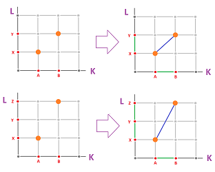
The illustration shows how we may be able to create a cubical map: $$g(AB):=XY,$$ by extending its values from vertices to edges. The extension succeeds (fist illustration) when $X=g(A),\ Y=g(B)$ are the end-points of an edge, $XY$, in $L$. When they aren't, the extension fails (second illustration); indeed, $XZ=g(A)g(B)$ isn't an edge in $L$. In that case, we may try to subdivide $K$, or, without subdivision, we can construct a chain for the value that we seek: $$g(AB):=XY+YZ.$$ The general idea is then to construct a chain map that approximates $f$.

Let's review why we didn't prove a cubical version of the approximation theorem along with the simplicial one.

First, the theorem that provides a continuity-type condition with respect to the cubical structure still holds:

Theorem. Given a map $f:|K|\to |L|$ of realizations of two complexes. Then there is such an $M$ that for every vertex $A$ in $K^m$ with $m > M$ there is a vertex $V_A$ in $L$ such that $$f(N_{K^m}(A))\subset N_L(V_A).$$

Second, just as with simplicial complexes, these vertices in $L$ serve as the values of a “cubical approximation” $g$ of $f$ -- defined, so far, on the vertices of $K$: $g_0(A)=V_A$. Then $$f(N_{K^m}(A))\subset N_L(g_0(A)).$$ The next step, however, is to extend $g$ to edges, then faces, etc. of $K$. Unfortunately, we can see below that for cubical complexes the analog of the Star Lemma that we need isn't strong enough for that.

Lemma. Suppose $\{ A_0,A_1 ,...,A_n \}$ is a list, with possible repetitions, of vertices in a cubical complex. Then these vertices belong to the same cell in the complex if and only if $$\bigcap _{k=0}^n N(A_k) \ne \emptyset.$$

Exercise. Prove the lemma.

In contrast to the case of simplicial complexes, here the condition doesn't guarantee that the vertices form a cell but only that they are within the same cell. Indeed, $A_0A_1$ may be the two opposite corners of a square. This is the reason why we can't guarantee that an extension of $g$ from vertices to edges is always possible. For example, even when $AB$ is an edge in $K$, it is possible that $g_0(A)$ and $g_0(B)$ are the two opposite corners of a square in $L$! Then there is no single edge connecting them as in the case of a simplex. However, a sequence of edges is possible. This sequence is the chain we are looking for.

Exercise. Prove that, for any map $g_0:C_0(K^m)\to C_0(L)$ with $$\{ AB\} \in K^m \Rightarrow g_0(A),g_0(B) \in \sigma\in L,$$ there is a map $g_1:C_1(K^m)\to C_1(L)$ such that together they form a chain map in the sense that $\partial _1g_1=g_0\partial_1.$ Hint: the cube is edge-connected.

Let's make explicit the fact we have been using; it follows from the last lemma.

Lemma. Under the conditions of the theorem, if vertices $ A_0,A_1 ,...,A_n$ form a cell in $K^m$ then the vertices $g_0(A_0),g_0(A_1) , ...,g_0(A_n)$ lie within a single cell $\sigma$ in $L$.

In the general case, the existence of such a chain follows from acyclicity of the cube.

Theorem (Chain Approximation Theorem). Given a map $$f:|K|\to |L|$$ between realizations of two cubical complexes. Then there is a chain approximation of $f$, i.e., a chain map $$g=\{g_i\}:C(K^m)\to C(L),$$ for some $m$, such that $$f(N_{K^m}(A))\subset N_L(g_0(A)),$$ for any vertex $A$ in $K$, and $|g(a)|$ lies within a cell of $L$ for every cell $a$ in $K$.

The proof is inductive. We build $g:C(K^m)\to C(L)$ step by step, moving from $g_{i}:C_i(K^m)\to C_i(L)$ to $g_{i+1}:C_{i+1}(K^m)\to C_{i+1}(L)$ in such a way that the result is a chain map: $\partial _{i+1} g_{i+1} = g_i\partial_{i+1}$.

Exercise. Sketch an illustration for $i=2$.

Each step is justified by the following familiar result that we present as a refresher.

Proposition. Suppose complex $Q$ is acyclic. Then $Q$ satisfies the following equivalent conditions, for all $0<i<k$:

• (a) $H_i(Q^{(k)})=0$;
• (b) every $i$-cycle is an $i$-boundary, in $Q^{(k)}$;
• (c) for every $i$-cycle $a$ there is a $(i+1)$-cycle $\tau$ such that $a=\partial \tau$, in $Q^{(k)}$.

Exercise. Provide the details of the proof of the theorem.

Exercise. Prove that two chain approximations, as constructed, are chain homotopic. Hint: use the proposition.

Then the homology map of $f:|K|\to |L|$ is well defined as the homology map of any of those chain approximations: $$f_*:=g_*:H(K)\to H(L).$$ The rest of the homology theory is constructed as before.

If we set the approximation problem aside, we can summarize the construction of the chains in the last part of the proof, as follows.

Theorem (Chain Extension Theorem). Suppose $K$ and $L$ are cell complexes and suppose $\alpha$ is a collection of acyclic subcomplexes in $L$. Suppose $g_0:K^{(0)}\to L^{(0)}$ is a map of vertices that satisfies the following condition:

• if vertices $A_0,...,A_n$ form a cell in $K$ then the vertices $g_0(A_0),...,g_0(A_n)$ lie within an element of $\alpha$.

Then there is a chain extension of $g_0$, i.e., a chain map $$g=\{g_i:\ i=0,1,2,...\}:C(K)\to C(L),$$ that satisfies the following condition:

• $g(a)$ lies within an element of $\alpha$ for every cell $a$ in $K$.

Moreover, any two chain maps that simultaneously satisfy this condition are chain homotopic.

This theorem will find its use in the next section.