See first Objects in binary images and Gray scale images.

1 Introduction

An image.

Its blurry version.

In binary images objects are either black areas surrounded by white background or white areas surrounded by black background. Similarly, our initial assumption about gray scale images will be that objects are either darker areas surrounded by lighter background or lighter areas surrounded by darker background. In other words, the dark objects are the connected lower level sets and the light objects are the connected supra-level sets of the gray level function. The boundaries of the objects are the level curves. Since all of these sets are connected collections of pixels they will be represented as 0- and 1-cycles.

At this stage the image analysis does not have unambiguous results because we don't know exactly where the boundaries of the objects are.

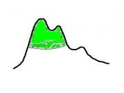
The visual inspection of the image reveals that it contains two dark objects. This information can also be acquired from the analysis of the frames of the image, as follows. The number of objects in each frame is: 1, 2, and 1. However, to avoid double-counting, we will only count an object if it does not have an ancestor in the previous frame. Then the total count of objects in the image is: 1 + 1 + 0 = 2. This is the maximum possible number. The user may decide that one or both of these objects are noise. In the latter case there is only one object – the whole square.

An image and its two objects.

The frames of the image.

An object is a lower level set of the gray scale function.

Preview the results of this approach here: Examples of image analysis.

2 Our approach

Objects in a gray scale image should be either connected darker regions surrounded by lighter background, or connected lighter regions surrounded by darker background. We choose the former.

The collection of all potential objects is acquired via Thresholding.

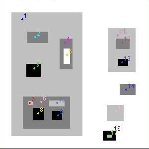
Note that objects should not be identified with flat areas, i.e., the areas where pixels have the same gray level. The approach is acceptable for binary images, but in case of gray scale images it would produce boundaries of objects (see also Boundaries in gray scale images). We are looking for areas where pixels have the same gray level or less. For example, in the image below all rectangles (including the interior) are objects. These are called the lower and upper level sets.

Of course, this principle produces too many objects. In the image to the right, some rectangles are contained in bigger ones. According to the above principle there are total of 17. However not all of them should be counted. To have the correct count of objects in a gray scale image, we will follow this principle.

If one object contains another, only one of them should be counted.

The principle is vacuously true for binary images. For gray scale images, the larger object is simply the background for the smaller one. An extreme case is when the larger object is the whole image. Clearly, it should not be counted.

This principle still leaves room for ambiguity. If only one of the two is counted, which one? More importantly, which one should be captured, measured, etc? The answer will be given by the user.

For example, objects that are too small or have too low contrast may be deemed unimportant. They are noise.

There is still some room for ambiguity. Should all objects that aren't noise be counted? No, because some of them may contain other objects. These objects represent the background for other objects.

The noise objects and the background objects are inactive. The rest are active.

Thus we have this rule:

3 Graph representation

The complete graph (only dark).

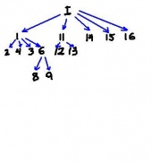
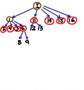
To illustrate consider the graph below. It describes the relation between all objects in the image - each object contains the one the arrow point at. 'I' stand for the object which is the whole image. For the sake of simplicity we ignore light objects.

Depending on the analysis setting, some of these objects will be

• active (circled with red),
• background (circled with brown), or
• noise (no marking).

Consider the two examples below.

• If there are no restrictions from the user (there is no noise), there are 14 objects - 10 dark and 4 light.
• If the user decides that everything smaller than say 500 pixels is noise, you are left with just 8 dark objects.

Analysis: 10 dark and 4 light active objects.

Analysis: 10 active (dark) nodes in the graph.

Analysis: 8 dark active objects.

Analysis: 8 active nodes in the graph.

The graph is a tree, which is called the inclusion tree. Using the standard terminology of graph theory,

• the whole image object is the root node,
• the noise nodes are found as a collection of sub-trees corresponding to nodes,
• the active nodes are leaf nodes of what's left after noise nodes have been removed,
• the background nodes are the rest.

For light objects the inclusion tree will look upside down. Dark and light trees wired together form the topology graph.

Exercise. Construct the inclusion tree for light objects in the above image.

Exercise. Is it possible to have two green (light) contours inside each other without a red (dark) one between them?

Some users have expressed the concern that the larger gray rectangle should also be counted because it's just another object behind the smaller ones. However, these are 2D images and there is no "behind" in 2D...

See also, Graph representation of images.

4 Where is the boundary?

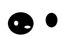
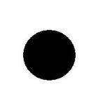
As another justification for our approach, consider this situation. The image with 255 concentric circles (rings) with growing - as you move from the center - levels of gray does not contain 256 objects; it's one dark object. The situation is illustrated below. The first image contains a black circle and the second its blurred version. In either image, there is only a single object. This is the case even though if you zoom in on the second image, it may appear that lighter objects stick out "from under" darker ones.

A black circle.

A black circle blurred.

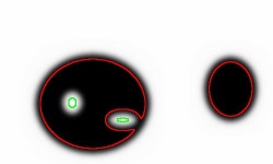
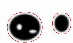
It may seem clear that in the above image there are two objects and the fist one has two holes. However, where the boundaries of these objects are located depends on the chosen threshold or thresholds. The choice of these thresholds will affect the topology of the image, as illustrated below.

75_10

75_119

75_250

670_127

The chosen thresholds will affect the measurements of the objects will also be different. As a result some of the objects may or may not be discarded as noise.

The maximal number of dark (light) objects is equal to the number of local minima (maxima) of the gray scale function.

Our approach to dealing with this ambiguity is to collect all possible cycles and then filter them based on size, contrast, etc.

The acquisition of all possible cycles is carried out via image thresholding. Given a number T, thresholding is the process of replacing all the pixels with gray level lower than or equal to T with black leaving the rest white. This creates a binary image that we call the frame corresponding to T. As gray runs from 0 to 255, we have a sequence of 256 frames. Observe that as you move from frame to the next, more black pixels appear.

There may be many characteristics that evaluate the importance of objects in terms of noise vs not noise. Some of the most important ones are discussed in Measuring objects.

To summarize, each level of gray can serve as a threshold and produce a binary image. Each of them is analyzed and a collection of binary objects is constructed. As the threshold grows these objects grow and merge. This creates a hierarchy (tree) of binary objects that we interpret as one or several “dark” objects in the image. Similarly, the white pixels form white objects for each threshold and eventually produce “light” objects. Of course, light objects may turn out to be holes in dark objects or vice versa. For more see Grayscale Images.

The remaining ambiguity is resolved in Pixcavator by means of sliders that allow you to choose limits on sizes and contrasts of the objects.

To experiment with the concepts, download the free Pixcavator Student Edition.