Images as functions of two variables

1 Binary images

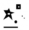
Binary image is a table of 0s and 1's. We treat each pixel as a square. The union of these squares gives us the domain of the function. This function has only two possible values.

2 Gray scale images

Grayscale Images are defined as follows. The level of gray of each pixel is given by a number between 0 and 255. Thus, there are the total of 256 = 2⁸ levels of gray. These numbers together form the gray scale function of the image. An example is on the right.

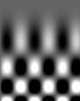
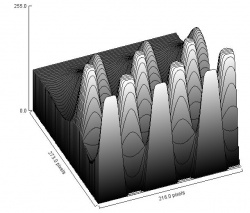
Another example with larger (162x205) image is below.

The image on the left is accompanied by its gray scale function. Lighter means higher values and darker means lower values.

See also Functions of several variables and Gray scale function.

3 Color images

Each pixel is associated with 3 numbers, so this is a vector function.

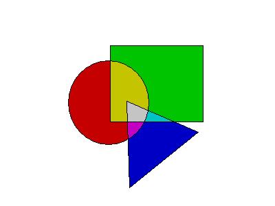
The color effect is achieved by combining different levels of red, green, and blue (RGB). Each color runs from 0 to 255. Thus, in an RGB image to every pixel there assigned 3 integers. One can think of a color image as a 3-vector attached to each pixel or as 3 tables of integers, etc. Our approach will be different. By means of a procedure similar to thresholding described above we represent color images as arrays of binary images. The color space is a 255×255×255 array with each entry corresponding to a particular color. As a result, thresholding a color image will produce a 255×255×255 array of binary images.

There also may be "multi-channel" images or images with other attributes assigned to each pixel...

4 Applications

Problem: Suppose we have a binary image. How do we compute the area of the region R of 1's (pixels are treated as squares)?

One can simply run through the image row by row and count 1's. However, this calculation is "expensive", given that

 time ~ N, number of pixels, and 
 not time (not) ~ n, number of pixels in the region R.

Further, it is possible that N >> n. On the other hand, following the boundary in the calculation is rather inexpensive as time ~ √n. To apply Stokes theorem, we treat the image as a function of two variables. This function is constant on each pixel, so it's integrable. Then

 ∫∫R 1 dA = ʃ∂R x dx,

and the integrals turn into sums:

 ∑i ∑j 1 = ∑x xk     for horizontal segments.
 where xk is the x-coordinate of k-th point.

The result is a simple algorithm (utilized in Pixcavator image analysis software).