This site is devoted to mathematics and its applications. Created and run by Peter Saveliev.
Lengths of curves
From Mathematics Is A Science
The article is about "digital curves". For lengths of continuous curves, see Arc length.
1 Problem
How do we measure the length of a curve in a digital image?
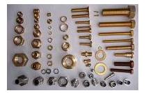
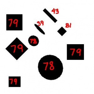
But first, why do we care? Consider this image.
Suppose we want use computer vision to count nuts and bolts separately. Suppose we have detected and captured these objects. We can find their areas. However, since some of these objects have about the same size in terms of the area, we have to look at their shapes. We want to be able to evaluate shapes of objects and the most elementary way to do it is to compare their areas to their perimeters. The ability to compute lengths becomes crucial.
Specifically, we use roundness of objects, which is $$Roundness = 4\pi \frac{area}{perimeter^2}. $$ The roundness will tell circles from squares and squares from elongated rectangles, as follows.
Two rectangles, same area -- very different roundness: 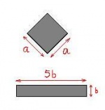
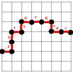
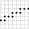
In binary images, objects appear as collection of pixels. Curves are represented as sequences of points.
Length of a digital curve:
It seems “obvious” that the length of the curve should be the total sum of distances between consecutive points. It is our concern however that the same “physical” curve will have different digital representations - depending on the image's resolution and the curve's orientation with respect to the grid. For the length to be a meaningful characteristic of the "physical" curve, all representation should have the same length – approximately. More precisely, as the resolution increases the lengths of the digital representations should converge to the "true" length of the curve.
In particular, the length should be independent from the orientation of the curve with respect to the grid of the image. As analysis below shows, this is not the case if we adopt this definition of length.
Exercise: Show that the area and other related characteristics of objects are independent of digital representation, in the above sense.
2 Initial approach
Let's take the direct approach first:
That's the way it is normally done...
Unfortunately, the curves we see on the screen aren't "real" - they all consist of sequences of pixels. The result is that the length of the "physical" curve and the length of its digital representation may be very different.
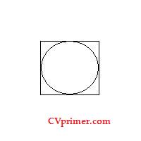
Here is a simple example: the perimeters of a square and the inscribed circle are the same!
(By the way, this implies that, $\pi=4$!) Indeed, it takes exactly as many vertical and horizontal steps to get from the left end of the circle to the top - no matter whether you make just one turn or many. The curve isn't really a curve...
Let's consider another example in more detail.
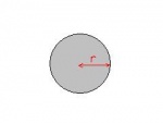
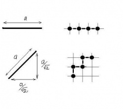
If r is the size of the pixel, a line segment of length a will be represented by roughly $a/r$ pixels… but only if it is placed horizontally or vertically!
If it is placed diagonally, there will be $\sqrt{2}a/r$ pixels arranged in the staircase pattern. So:
- Horizontal orientation: length $= a$;
- Diagonal orientation: length $= \sqrt{2}a = 1.42a.$
Conclusion: the length depends on the orientation of the curve with respect to the grid of the image.
The result is that the digital length of a curve may vary by 40%.
It is natural to try to deal with this problem the same way one would deal with other accuracy problems -- by increasing the resolution of the image. In fact, a curve can be approximated by a digital curve with any degree of accuracy (see Approximating paths).
Unfortunately,
Exercise. Why?
Ignoring the error may be dangerous.
The roundness is supposed to be lower for elongated objects, like bolts. This works perfectly well in the continuous domain but in the digital domain it is possible to think of very different shapes with both area and perimeters exactly same.
- Diagonally oriented square with side a:
- area $= a^2$,
- perimeter $= 4\sqrt{2}a$.
- Horizontally oriented rectangle with sides $b=(\sqrt{2}-1)a$ and $b'=(\sqrt{2}+1)a=5b$:
- area $= a^2$,
- perimeter $= 4\sqrt{2}a$.
Thus, a horizontally oriented rectangle with proportions about $1$-to-$5$, just as in the image above, will have the same measurements as a diagonally oriented square. We can't tell a bolt from a nut…
3 Analysis
Let’s review. Computing lengths of horizontal and vertical segments produces correct results. Computing lengths of diagonal segments leads to a 40% error.
Solution is to break a curve into "short" curves:
Note: MATLAB's regionprops functions computes the perimeter this way, as the number of pixels in the boundary.
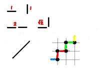
A possible solution may be to break the curve into larger pieces. Every time we have a triple of consecutive points arranged in a triangle we should replace $1+1=2$ in the computation with $\sqrt{2}$. The result is that now, at least, all $45$ degree segments have correct lengths!
But what about $30$ degree segments? Consider segments with 2 horizontal steps followed by 1 vertical. Then
- “True” length $= \sqrt{2^2+1^2} = \sqrt{5} = 2.24. $
- Old method: length = $3$.
- New method: length $= 1+\sqrt{2} = 2.41$.
The error is still almost 8%!
Note: In the last computation, the length of a single 3 step segment $= 1/2$ the length of two $3$ step segments $= 1/2(2+\sqrt{2}+\sqrt{2}) = 1+\sqrt{2}$.
This error appears to be commonly accepted (often without discussion or even disclosure). For example, in ImageJ, a square rotated to $30$ degree has roundness (circularity) equal to $70$, instead of $80$ (Pixcavator produces a similar result).
Exercise. If the relative error for the length is $n$%, what is the relative error for the roundness?
"Short" curves used as building blocks:
Now we need to take into account this new type of segment. Then we have three types: horizontal/vertical, diagonal, and now $2$-straight-then-turn (same length as "diagonal"). To compute the length of a curve we break it into segments of the three types and add their lengths.
Next we try an angle between $0$ and $30$ degrees – there will still be an error. And so on. This suggests that there is no exact method to compute the length by breaking it into smaller pieces. This is the conclusion of the paper On Local Definitions of Length of Digital Curves [1] by Mohamed Tajine and Alain Daurat.
Extended analysis:
- one breaks a digital curve into a sequence of $n$-step curves,
- each curve is assigned a length (it does not have to be the distance from the beginning to the end), then
- the length of the original curve is the sum of those.
As the resolution approaches $0$, the length computed this way should converge to the “true” length. The paper proves that in general it does not! The relative error remains the same regardless of the resolution.
The conclusion is the following:
...by traversing it only one time. And
A simple "explanation" again: once $n$ is chosen, the number of possible angles that curves of $n$ steps can generate is finite. Meanwhile slopes of segments run (continuously!) from $0$ to $360$ degrees. No matter how large $n$ is, there will be whole intervals of possible slopes missed...
Computing software, such as MATLAB and OpenCV, can also compute lengths by curve fitting. This approach, however, faces the same issue. Indeed, you either take into account all points, which may be unfeasible, or you sacrifice the accuracy.
The problem discussed here falls in the category of Robustness of geometry. A similar issue will arise when you compute the Surface area.
4 A brute force solution
As $n$, the number of steps in the curves in the decomposition, increases, the accuracy improves.
This is a good news because it allows one to produce meaningful results in shape evaluation. If you know the accuracy that will be appropriate in your application, you can choose $n$ that will guarantee it.
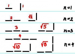
This is how the problem is solved:
- Given $n$, we build the collection of all $n$-step curves.
- Each $n$-step curve is assigned a length equal to the distance from the beginning to the end.
- A given digital curve is represented as a sequence of $n$-step curves (plus possibly one shorter) glued together end to end.
- The length of this digital curve is assigned to be the sum of lengths of these curves.
It is clear that all it takes to compute the length is a single run along the curve.
The computation of roundness is implemented in Pixcavator. The algorithm takes into account the number of steps (perimeter) and the number of turns (curvature). This is sufficient for exact computation of lengths of both horizontal/vertical and diagonal segments.
Exercise. Suggest a formula for the "adjusted" perimeter as a combination of perimeter and curvature.
The image above is an example of computation of roundness with Pixcavator.
First thing to notice is that the roundness of squares is independent of their orientation. Large squares have roundness close to $80$. Because of the error of the computation of the perimeter, so do large circles. Nonetheless, in spite of this error Pixcavator successfully distinguishes between circles/squares and elongated objects.
The roundness starts to distinguish circles ($90$) and squares (still $80$) as they get larger ($600 \times 600$). For more examples, see Roundness.
5 Theoretical aspects
I tried to explain the reason for the failure above.
A broader explanation is that the geometry of the universe is independent of direction, i.e. isotropic. By adding the grid and limiting our curves to it we make our approximation of this universe anisotropic. As the examples show, the horizontal and vertical directions are different from the rest. And no matter how much we improve this approximate universe by making the grid finer and finer, it will remain anisotropic. Choosing a triangular or hexagonal grid or other tricks won't help.
The result is counter-intuitive. Indeed, refining the approximation has to lead to the exact result. Actually, there is a moment in calc1, when the issue arises and it requires some careful thinking.
The issue comes up when the definition of the Riemann integral is introduced. The integral is defined as the "limit" of Riemann sums, but what sums? They may be initially defined as a sums over intervals of equal length. In this case there is only one parameter and it may seem that you are just dealing with the same limits as the ones used for continuity, derivatives etc. However, this definition is inadequate if you want to prove some simple properties of the integral. Turns out, you need to be able to deal with partitions of the interval into arbitrary sub-intervals. Then the Riemann integral is still a limit but it's the limit of Riemann sums over all possible subdivisions of the interval. The issue is often glossed over in a standard Calculus class (so that not to traumatize the students).
A similar situation here. We need to consider all possible rectangular grids. Then take the limit. The limit will be a two-parameter kind: the width of the pixel and its height go to 0, independently. Then, when both are smaller than some $\delta$, the length of the approximated curve will be within some given $\epsilon$ from the length of the "real" curve.
Exercise: How do we use this insight to improve the accuracy?
Note: One might wonder why this doesn't work because we know from calculus that the arc-length of a curve is defined and computed via approximation of the curve by line segments. The difference is that the end points of these segments lie exactly on the curve and all slopes are possible!
A similar issue arises PDEs are approximated in the context of Discrete exterior calculus, such as heat equation, etc...
For other ways to measure objects see Measuring objects.
Digital discoveries
- Casinos Not On Gamstop
- Non Gamstop Casinos
- Casino Not On Gamstop
- Casino Not On Gamstop
- Non Gamstop Casinos UK
- Casino Sites Not On Gamstop
- Siti Non Aams
- Casino Online Non Aams
- Non Gamstop Casinos UK
- UK Casino Not On Gamstop
- Non Gamstop Casino UK
- UK Casinos Not On Gamstop
- UK Casino Not On Gamstop
- Non Gamstop Casino UK
- Non Gamstop Casinos
- Non Gamstop Casino Sites UK
- Best Non Gamstop Casinos
- Casino Sites Not On Gamstop
- Casino En Ligne Fiable
- UK Online Casinos Not On Gamstop
- Online Betting Sites UK
- Meilleur Site Casino En Ligne
- Migliori Casino Non Aams
- Best Non Gamstop Casino
- Crypto Casinos
- Casino En Ligne Belgique Liste
- Meilleur Site Casino En Ligne Belgique
- Bookmaker Non Aams
- カジノ ライブ
- онлайн казино с хорошей отдачей
- スマホ カジノ 稼ぐ
- ブック メーカー オッズ
- Top 3 Nhà Cái Uy Tín Nhất
- Trang Web Cá độ Bóng đá Của Việt Nam
- Casino En Ligne Avis
- Casino En Ligne France
- Casino En Ligne
- 꽁머니 토토
- Casino Online Non Aams
- Meilleur Casino En Ligne
- Casino En Ligne France Légal
