This page is a part of CVprimer.com, a wiki devoted to computer vision. It focuses on low level computer vision, digital image analysis, and applications. It is designed as an online textbook but the exposition is informal. It geared towards software developers, especially beginners, and CS students. The wiki contains mathematics, algorithms, code examples, source code, compiled software, and some discussion. If you have any questions or suggestions, please contact me directly.
Image processing
From Computer Vision Primer
To make this wiki as self contained as possible we include a few elementary facts about image processing.
The list is very short because we are interested in the analysis of an image “as is”. We will not try to read the mind of the user and try what he wants to do with the image. We will not discuss image acquisition, translation of analog information into digital, or representation of 3D objects by 2D pictures, or the nature of the image or the noise. More on that elsewhere.
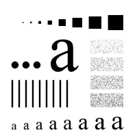
Binary images are tables of 0s and 1s. Normally, 0s correspond to black pixels and 1s to white. The pixels typically represent the black object on the white background.
To avoid confusion and stay mathematically consistent we avoid referring to images as matrices. The reason is that we will not perform algebraic operations with images. Matrices will appear elsewhere in the context of homology theory.
Gray scale can be represented by a number between 0 and 1. In practice, however, gray scale images are tables of integers. The integers normally run from 0 (black) to 255 (white).
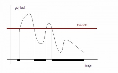
Thresholding is the following procedure:
Given a number, threshold, T between 0 and 255,
create a T-th frame by replacing all the pixels
with gray level lower than or equal to T with black (0),
the rest with white (1).
Converting a gray scale image to a binary image is a common technique in image analysis. By thresholding of a gray scale image normally is understood the following procedure. Given a number, threshold, T between 0 and 255, create the binary image by replacing all the pixels with gray level in the original image lower than or equal to T with black.
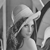
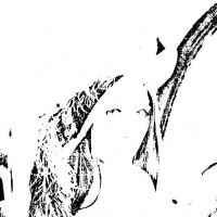
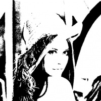
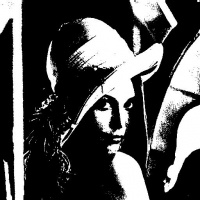
As you raise the threshold, the number of black pixels increases, as in the images above.
For more see Thresholding.
Dilation is an operation that makes black each pixel adjacent to black. Erosion makes white each pixel adjacent to white. By adjacent we understand a pixel that shares an edge with the given pixel. Alternatively, it may be a pixel that shares a vertex. For the intended purpose the difference may be ignored.
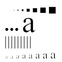
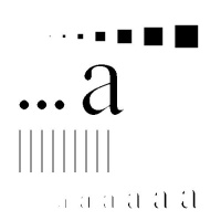
For more see Dilation and erosion.
The color effect is achieved by combining different levels of red, green, and blue (RGB). Each color runs from 0 to 255. Thus, in an RGB image to every pixel there assigned 3 integers. One can think of a color image as a 3-vector attached to each pixel or as 3 tables of integers, etc. For more see Color Images.
Videos are treated simply as sequences of still images. Since each frame is a color image represented as a 3-parameter array of binary images, the whole video is a 4-parameter array of binary images. The extra parameter is time. In the simplest case of a binary video it is a sequence of binary images just like a gray scale image. This similarity will be exploited in the forthcoming articles. For more see Image Sequences.
3D binary images are 3-parameter arrays of 0s and 1s. The volume elements are called voxels. In the same fashion as above 3D gray scale images are represented as sequences of 3D binary images.
In some industries 3D images are acquired by scanners. The result is not a collection of black and white voxels on a grid but a disorganized point cloud. To find the object represented by the point cloud the points have to be connected by edges, triangles, and, in 3D, tetrahedra. To find which points should be connected, balls are grown around each of them (just like dilation) until they start to intersect. The result is called a triangulation. How exactly this is done is not discussed in here. However, these objects will also be the subject of our analysis.
Another source of alternative formats is mapping industry. The maps are created of such simple geometric shapes as triangles, trapezoids, etc. The methods put forward in this wiki apply to geometric figures of arbitrary shape called cells. For more see Cell decomposition of images.
See also Pixcavator's image processing tools. Download the free Pixcavator Student Edition here.
Consider other Fields related to computer vision.
Digital discoveries
- Casinos Not On Gamstop
- Non Gamstop Casinos
- Casino Not On Gamstop
- Casino Not On Gamstop
- Non Gamstop Casinos UK
- Casino Sites Not On Gamstop
- Siti Non Aams
- Casino Online Non Aams
- Non Gamstop Casinos UK
- UK Casino Not On Gamstop
- Non Gamstop Casino UK
- UK Casinos Not On Gamstop
- UK Casino Not On Gamstop
- Non Gamstop Casino UK
- Non Gamstop Casinos
- Non Gamstop Casino Sites UK
- Best Non Gamstop Casinos
- Casino Sites Not On Gamstop
- Casino En Ligne Fiable
- UK Online Casinos Not On Gamstop
- Online Betting Sites UK
- Meilleur Site Casino En Ligne
- Migliori Casino Non Aams
- Best Non Gamstop Casino
- Crypto Casinos
- Casino En Ligne Belgique Liste
- Meilleur Site Casino En Ligne Belgique
- Bookmaker Non Aams
- カジノ ライブ
- онлайн казино с хорошей отдачей
- スマホ カジノ 稼ぐ
- ブック メーカー オッズ
- Top 3 Nhà Cái Uy Tín Nhất
- Trang Web Cá độ Bóng đá Của Việt Nam
- Casino En Ligne Avis
- Casino En Ligne France
- Casino En Ligne
- 꽁머니 토토
- Casino Online Non Aams
- Migliori Casino Non AAMS
- Meilleur Casino En Ligne
- Casino En Ligne France Légal
- Casino En Ligne France Légal
- Casinos En Ligne
- Mejores Casinos Online
