This page is a part of CVprimer.com, a wiki devoted to computer vision. It focuses on low level computer vision, digital image analysis, and applications. It is designed as an online textbook but the exposition is informal. It geared towards software developers, especially beginners, and CS students. The wiki contains mathematics, algorithms, code examples, source code, compiled software, and some discussion. If you have any questions or suggestions, please contact me directly.

From Computer Vision Primer

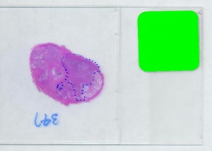
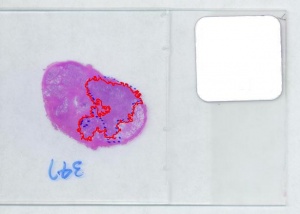
The first picture explains what normally happens when a prostate tumor has to be evaluated. The prostate is cut into thin slices and the slices are put on pieces of glass. Next, the doctor outlines the tumor within the prostate with a marker. Finally, the area of the outlined region is evaluated in each slice and the volume of the tumor is estimated.

Evaluating the area of the tumor with a naked eye will give you a very low accuracy. Best one can do to improve that is to superimpose a grid over the image and count the number of squares that fall into the tumor. Then the accuracy will be inversely proportional to the size of the square but the smaller the square the more complex the manual counting will be.

Digital image analysis is a necessity here.

I analyzed the shrunk version (615x439) of the image with Pixcavator followed by some back-of-the-envelope calculations.

The critical part of analysis is the calibration. For that I used the square label in the image. It is known that its side is 2.2 cm. Now, I pushed the size slider almost all the way to the right and ended up with just one object -the label (green). Its area according to the table is 29,516 pixels. If we ignore the round corners (introducing some error here, unfortunately), it is a square. So 29,810 pixels = 2.2 * 2.2 = 4.84 sq cm.

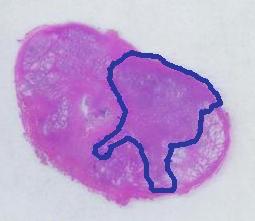
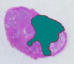
Next, the tumor. The dotted line is made solid using MS Paint. The you run Pixcavator. The contour has the area of 9,491 pixels. So, it is 9,491 * 4.84 / 29,810 = 1.54 sq cm.

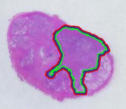
There is still the issue of error however. The error produced by hand drawing is estimated in the next experiment. Pixcavator evaluated the area on the outside of the curve (9,774) and on the inside (7,112). Hence the area of the curve is (9,774 – 7,112) / 9,774 = 27% of the outside of the tumor. That's the error.

It seems too high!

To verify the result, let's approach from another direction. The perimeters are 542 and 530 respectively. Then the average thickness of the line is (9840-7342)/536 = 4.7 pixels. Examination of the image confirms this number. Of course, the error can be easily cut down by making the line 1/2 thinner… To be fair the error should be divided by 2.

That brings us to the possibility of discovering the tumor within the prostate automatically. To be precise, the procedure would be semi-automatic not automatic, and it is the doctor who would make all the decisions. He chooses the contours and Pixcavator just counts pixels. What it gives you is a procedure that is somewhat simple – moving sliders until you have a good fit – and quite accurate – if the fit is good. Finding a good contour won’t require training but just a bit of practice. The last image shows that this approach isn’t totally unreasonable…

Other case studies