This is an example of “electron micrographs of biological membranes containing proteins. We need to get as much as possible information about the particle size, shape, clustering, crowdiness, etc.”

I ran Pixcavator with both images. The quality of the first one is much better and so are the results. The particles are captured quite well and with a couple minutes of trial and error they could be even better. Once the contours are found, the information about sizes, shapes, locations is provided (table on the right). The results for the second image are less encouraging. The shadows are just too large relative to the sizes of the particles so that their borders aren’t well defined. The result might still be OK for counting, as well as locations and distances.

You can find all info about the table in this article Pixcavator’s output table. Some examples relevant to this task are here Particle and cell analysis.

“Can the histograms of the size/diameter distributions be calculated?”

Yes, but only via Excel (another example: Measurement statistics of fibers). The table contains the centers of mass of all particles and one can easily compute the distances between them (if you want to treat the particles as circles, you subtract their radii). Also, the Voronoi diagram is intended exactly for such a problem.

A much simpler, but cruder, way would be to assume that the particles are evenly distributed. You can compute the average distance by looking at the density of particles (number of particles / the area of the image). Also you can think of them as circles, then, for example, if you have 100 particles in a 100×100 image, the average distance to the nearest neighbor is 10.

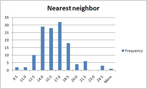
For clustering, I did some work with the data. Instead of dealing with a fairly complex geometry of Voronoi diagram, I implemented a very simple statistical computation, with Excel: the distribution of the distance to the nearest neighbor. The spreadsheet is here. The Excel work was awkward - for example I had to transpose a column. I wish I knew Excel better to come up with something more straightforward. The result seems to make sense:

Other examples of image analysis

A request came from a researcher who wants to “analyse images from optical microscopy of surfactants. Those images have a hair of known thickness in order to obtain an idea of the real dimensions involved… The hair’s thickness is 0.045 mm.”

I did some preliminary work. First you need to convert pixels into millimeters. I re-analyzed the image. I had to add a black border to the image. This is a way to capture a light object that touches the edge of the image (another is to invert the colors).

and the thickness of the hair is 23 pixels. So, 23 pixels = .045 mm, or 1 pixel = .045/23 = .002. This is the conversion factor (aka calibration factor). I inserted it at the top the output table. On the right you see two new columns - they are the sizes and the perimeters converted into mm.

One would have to repeat the analysis of the hair thickness for all images though, unless all pictures are taken at the same distance and the hair is the same. If these images are taken from the same distance, you need to do the calibration only once and then use the same conversion factor for all of them. Another good new is that the conversion procedure will work equally well regardless of 10X, 5X etc magnification that comes from the microscope.

See also other examples of image analysis