December 13, 2012
The contents of this blog are now a part of a book draft called Applied Topology and Geometry.
Comments Off
November 29, 2011
I started reading about this very recently but so far all makes a lot of sense.
The mathematics is both solid and interesting, especially stochastic calculus. This is a nice break from my recent experiences with what I would call “the mathematics of computer science”: computer vision and image analysis, machine learning, pattern recognition, and my favorite, PageRank.
One issue in this area I have been wondering about is the importance of randomness.
Consider these graphs:
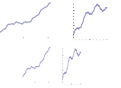
They seem similar to random fluctuation of stock prices which are supposed to follow the random walk model:

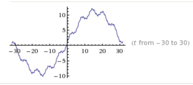
But, in fact, the curves are made of just five (5!) sine functions:
sin(t)+10sin(.1t)+.1sin(10t)+5sin(.2)+.2sin(5t):
It is interesting how everything is connected. A very important person in this field was Kenneth Arrow. He proved Arrow’s Impossibility Theorem, which is about voting, therefore, related to the ranking problem and PageRank. It is also related to the price equilibrium issue. Meanwhile, the existence of equilibria is frequently is addressed via fixed point theory — the topic of my thesis.
Comments Off
October 23, 2011
To experiment with ideas like this I’ve created this little spreadsheet. The formula comes from the original Page/Brin paper from 1998.
Suppose we have these ten “pages”: A, B, …, J. They are listed in the table as both rows and columns. The links are the entries in the table.
First we suppose that they link to each other consecutively: A → B → C → … → J.
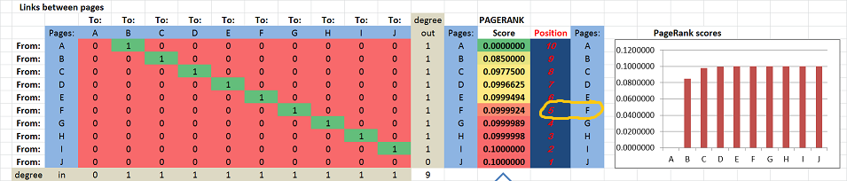
The PageRank scores, as well as the positions, of the pages are computed and displayed on the right. The scores for A, …, J are increasing in the obvious way: from 0 to .1. In particular, F is #5.
Next, suppose F adds a link to A: F → A. You can see that 1 has appeared in the first column of the table:
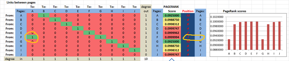
Now, suddenly F ranks first!
Yes, adding an outbound link has brought this page from #5 to #1.
The result certainly goes against our intuition. It shouldn’t be surprising though considering other problems with the math of PageRank.
This isn’t a new discovery of course. These are just a couple of references for you:
- The effect of new links on Google PageRank by Konstantin Avrachenkov and Nelly Litvak, Stochastic Models, 22:319–331, 2006.
- Maximizing PageRank via outlinks by Cristobald de Kerchove, Laure Ninove, and Paul van Dooren, Linear Algebra and its Applications 429 (2008) 1254–1276.
The conclusion is that the appearance of a cycle is what seems to be the reason for this behavior…
You won’t get a straight answer from Google on this. When asked to explain what PageRank is, they say it’s hardly a secret and refer you to the 1998 paper (or rehash its contents like here). However, if you criticize those ideas, the answer is: it’s irrelevant because PageRank isn’t that anymore, it is now composed of 200 various “signals”. So, what’s PageRank anyway? Glad you asked, it’s all explained in that paper from 1998…
Another cycle.
Comments Off
October 6, 2011
…for researchers who use and credit Pixcavator in their publications.
This is a new promotion: authors can get a year subscription (value of $245) for free, if they they credit our image analysis software in their publications.
So far we are aware of 30 such papers, in an amazing variety of fields.
Details of the offer:
- The paper should
- acknowledge the use of the software: “Pixcavator by Intelligent Perception”, and
- cite one of our papers: Pixcavator’s references (optional).
- The author should contact us with:
- the exact reference to your paper, and
- a paragraph-long quote from the paper about how Pixcavator was used (along the lines of Image analysis examples).
- We will send you a coupon to be used during purchasing (some charges may apply).
- The offer applies to: one per publication per author per year.
Comments Off
August 28, 2011
Gotcha! You thought this is about SEO. No, I meant “exist” in the mathematical sense…
When an entity or a concept in mathematics is introduced via a description instead of a direct computation, there is a possibility that this entity doesn’t even exist. This happens when there is nothing that satisfies the description. For example, “define x as a number that satisfies equation x+1=x” produces nothing.
Similarly, when something is introduced via an iterative process instead of a direct computation, does it always make sense? It’s possible that no matter how many iterations you run, you don’t get anything in particular (“divergence”). For example, “start with 1, then add 1/2, then add 1/3, 1/4, etc” leads to unlimited growth with no end.
So, what does this have to do with PageRank?
Let’s review the math behind it. Suppose  are the are the  pages/nodes in the graph (of the web). Suppose also that pages/nodes in the graph (of the web). Suppose also that ") is the PageRank of node is the PageRank of node  and together they form a vector and together they form a vector  . Then the ranking satisfy the “balance equation”: . Then the ranking satisfy the “balance equation”:
 = d \sum_{p_j \in S(p_i)} \frac{R (p_j)}{L(p_j)} + \frac{1-d}{N},")
where
*") is the set of nodes that (inbound) link to , is the set of nodes that (inbound) link to ,
*") is the number of (outbound) links from node is the number of (outbound) links from node  . .
Skipping some algebra here, we discover that the PageRank vector is found as:
 \left( \frac{1}{d}I-M \right) ^{-1}R_0,")
where the matrix  is is
 & \mbox{if }p_j \in S(p_i),\ \\ 0 & \mbox{if }p_j \notin S(p_i), \end{cases}")
and  = \frac{1}{N},i=1,2,\ldots ,N,") is the initial distribution of rankings. is the initial distribution of rankings.
Problem solved! But before we start celebrating we have to make sure that the inverse matrix in the formula exists!
The Perron–Frobenius theorem ensures that this is the case — but the matrix has to be “irreducible”.
Matrix is irreducible if and only if the graph with an edge from node  to node to node  when when  is ”strongly connected”, i.e., there is a path from each node to every other node. is ”strongly connected”, i.e., there is a path from each node to every other node.
But we all know that there are always pages with no inbound links! The proof fails.
So, we have no reason to believe that a PageRank distribution exists for the given state of the web. This means that, no matter how you compute , what comes out will be garbage.
Well, some people aren’t worried about this. Others worry so much that they try to fix it, in ridiculous ways. A common approach, for example, is to add “missing” links. Don’t get me started on that. If you introduce made-up parameters or try to make data fit your model, that’s bad math!
Are there other mathematical problems with PageRank? Still to come.
Comments Off
August 23, 2011
Summer is over and I would like to report on a student’s research project that I especially liked. The full title is of the project was
Modeling Heat Transfer on Various Grids with Discrete Exterior Calculus by Julie Lang.
The main issue we ended up studying was isotropy as heat is supposed to transfer equally in all directions. Since no grid is isotropic, this is a big issue. Every time, we would start with all the initial heat concentrated in a single cell and then saw if, after many iterations, the shape of the heat function is circular. If it wasn’t, the model was simply wrong! Every time we had to come up with a modification and then continue with trial and error. Not very rigorous but fascinating scientifically. The last grid was rhomboidal and we were left with an oval, unfortunately…
It’s a good story and an interesting read. This is the link to the project page.
Comments Off
August 2, 2011
Every time I get to read more about PageRank I run in serious issues with its math (previous posts here and here).
Briefly, the probabilistic interpretation of PageRank is invalid.
According to Brin/Page paper from 1998, “The probability that the random surfer visits a page is its PageRank.” And “We assume page A has pages T1…Tn which point to it (i.e., are citations). The parameter d is a damping factor which can be set between 0 and 1… Also C(A) is defined as the number of links going out of page A. The PageRank of a page A is given as follows:
PR(A) = (1-d) + d (PR(T1)/C(T1) + ... + PR(Tn)/C(Tn))
Note that the PageRanks form a probability distribution over web pages, so the sum of all web pages’ PageRanks will be one.”
When I decided to implement the PageRank algorithm a few days ago, I quickly discovered that it should be (1-d)/n instead of (1-d). That’s a typo, fine. But, after fixing this, I wasted half a day trying to figure out why the ranks still wouldn’t add up to 1. Turns out, it was all a lie: they don’t have to!
I don’t understand now how I missed that. If there is only one page, its PageRank has to be 1-d. If there are two pages with T linked to A and nothing else, then we can assign: T=0 and A=(1-d)/2. They don’t have to add up to 1!
Best one can say is this. If one uses the above formula for iteration and starts with a distribution, then yes, you will get a distribution after every iteration… But only if there are no link-less pages!
To get out of this trouble, there have been some tweaks suggested. Hard to tell which one is sillier:
- normalizing (dividing by the sum of all PageRanks) and
- assuming that no links means that the page links to every page.
That’s what happens when you try to make data fit the model.
After more than 10 years of usage, PageRank’s paradigm is clear. The people who care about their PageRank – millions of web site owners – understand what it is about. It isn’t about probability. PageRank is about passing something valuable from a page to the next along its links. This something has been called popularity, significance, authority, “link juice”, etc.
So, PageRank shows who, after all this “redistribution of wealth”, ends up on top. This seems to make quite a lot of sense, doesn’t it?
Unfortunately, the actual computations lead to problems.
In the presence of cycles of links, the algorithm diverges to infinity. This lead to the introduction of the damping factor (bad math), which didn’t prevent the gaming of the algorithm. Google’s answer was surreptitious tweaking, attempts to evaluate the “quality” of sites, manual interventions, on and on.
Even though this problem certainly isn’t a new discovery, the myth clearly lives on: Wikipedia says “PageRank is a probability distribution used to represent the likelihood that a person randomly clicking on links will arrive at any particular page.” It then proceeds to give an example in the next section that isn’t a distribution.
I’ve learned my lesson: bad math simply doesn’t deserve mathematical analysis. Once it’s determined that the idea is bad math, you know it’s a dead end! Instead, try to find an alternative. The acyclic rank still to come…
Comments Off
July 22, 2011
The multi-stage procedure is completed:
- prepare for the lecture by creating the initial notes;
- deliver the lecture (with a tablet) which always ends up very different from the textbook or the notes;
- save the notes as a Journal file (and also in pdf, for the web);
- edit the Journal notes: rewrite in full sentences to make the text more readable, clean up illustrations, proofread;
- transcribe the notes into TeX, put the result online with illustrations inserted;
- edit this text: make it more narrative, improve formatting, add links, proofread again.
The whole procedure is more time consuming than I expected initially. Stage 5 is especially hard and has required help (thanks Tom!). Stage 7 should be further polishing and more proofreading. I hope one day to be able to add stage 8: make the illustrations more professional.
Besides Calculus 1, other courses are at various stage of completion:
Comments Off
July 15, 2011
I will be attending the 23rd Canadian Conference on Computational Geometry held in Toronto, August 10-12, 2011.
I’ll give a talk called Robustness of topology of digital images and point clouds.
Abstract. Such modern applications of topology as digital image analysis and data analysis have to deal with noise and other uncertainty. In this environment, the data structures often appear “filtered” into a sequence of cell complexes. We introduce the homology group of the filtration as the group of all possible homology classes of all elements of the filtration, without double count. The second step of analysis is to discard the features that lie outside the user’s choice of the acceptable level of noise.
Comments Off
July 5, 2011
My previous post on the subject was “PageRank is an abomination (mathematically)”. My thesis was:
PageRank, as described by Google, is bad math.
Why? It appears that initially they made an arbitrary choice of the damping constant even though the choice affects the rankings.
The parameter is made-up and hidden from the user.
What has happened since, I don’t know. It’s a secret. I certainly haven’t heard an alternative story so far. And I can rely only on how it is described by Google – in the original papers and on their site. Below is a summary of the reaction to my post.
Re-reading the discussion, I can see now how many times I was distracted from my thesis by the “Google search works great” argument. I should’ve just replied: “PageRank is bad math. Please comment.” I admit though, I went beyond my main thesis and conjectured that PageRank’s problems are the cause of the problems of the whole search algorithm. I’ll try to make a case for that in a future post.
The response at Reddit was mostly along the lines: “The article is terrible, because Google search works great.” A surprising reaction to my thesis. Digging a bit deeper I realized that these people:
- love Google;
- assume that Google search == PageRank (or think that I do);
- think that “bad math” means 1+1=3.
The crowd is “technical”, I suppose. So, #1 is understandable, but #2 is not, while #3 is very, very common.
The praise for Google was very homogeneous:
“PR-based algorithms seem to work (very) well in the real world”; “yield very good search results”; “Google’s search algorithm works amazingly well”; “Google’s algorithm works extremely well”; “The page rank algorithm is actually extremely impressive, and obviously works well.”
What I see is that this attitude has shown cracks recently. There have been public complaints about Google search results: the JCPenney story, content farms, scrapers, Google’s own properties ranked above others, etc. These are recent complains from site owners about the Panda update. And just because Google dominates other search engines, also based on the PageRank idea, doesn’t make it good math.
There were other arguments against my thesis.
“[H]is main concern is over the fact that Google arbitrarily picked a constant for the decay factor, but that’s not actually a bad thing, and is done all the time in mathematical modeling… in no way upsets me as a mathematician.”
Reddit is anonymous by default, so I don’t know… A mathematician would ask about the effects of such a choice and try to prove (or disprove) that there isn’t any. Unfortunately, the choice does affect the order of pages that you get as the referenced paper indicated. As for the “all the time” comment, so what? If you do that, to me it means that you can’t come up with a better model (I think there is a way).
“[T]he graph used in the paper [that shows dependence of the rankings on the damping factor] is fairly contrived, and we’re mostly interested in what the algorithm does on real-world data.”
A fair point but one still has to ask for some evidence. Is there a case study where a large number of websites are analyzed and it is shown that changing the damping factor DOES NOT significantly affect the ranking of these sites? Well, at least this person didn’t claim to be a mathematician… I have to add then that even such a study wouldn’t resolve the bad math issue. What would? You’d need to
- define a class of graphs, let’s call them non-contrived;
- prove that the PageRank of a non-contrived graph is independent of the damping factor (or at least the top results aren’t);
- provide evidence that the Internet, now and in the future, is non-contrived.
“Pagerank is a starting point; it provides a rough sketch of page importance which is fine tuned by other more specific algorithms”.
Let’s consider this analogy: π =3 is bad math, but it’s “a very good starting point” for solving many real life problems. For example, you can build a hut, no problem. But what if you want to do something more sophisticated like building an airplane? With π =3 your plane will drop like a brick. And this will keep happening, no matter how much you fine tune your engineering. Suppose now that you replace π =3 with π = 3.14159265358979. OK, you’ve replaced bad math with better math, or maybe even good enough math (you can build your plane now). But π=3.14159265358979 is a time bomb! Sooner or later it will fail you when it’s not accurate enough anymore. Sooner or later you will need to understand what π is. Sooner or later you will need good math… (Is this what’s happened to Google?)
More to come…
This stuff will end up in the main site under PageRank and, yes, Bad math.
Comments Off
June 27, 2011
We are announcing the new release of our popular image analysis software.
In a new release we usually fix several bugs and improve the performance. There are a few improvements coming but this time the main news is our switch to the new activation provider for Pixcavator, RegNow. All new purchases will go through them from now on. There are a few tricky issues to take care of but we will do all we can to make the transition as painless as possible. Protexis will still be responsible for all old accounts.
The new purchase page is here.
Comments Off
June 23, 2011
I am working on several ebooks based on the courses presented in this site: see Courses. There are about 20 of them right now at different stages of completion. They will range from pre-calculus and up, all the way.
If you would like to be notified when they are ready, please fill this form.
Comments Off
June 14, 2011
Google released the new version of its image search. The screenshot speaks for itself:

For others see Visual image search engines.
Comments Off
May 29, 2011
My recent interest in data analysis has lead me to read about its uses in Internet search, then to Google search algorithm, then finally to its core, the PageRank.
PageRank is a way to compute the importance of web-pages based on their incoming and outgoing links.
PageRank is a mathematical idea that “made” Google’s web search algorithm. In fact, PageRank was the search algorithm, initially. Even with so many things added, PageRank remains the cornerstone of web search. Therefore, its problems become problems of web search and, hence, our problems. These problems, I believe, are mathematical in nature.
As a mathematical idea I find PageRank very unsatisfying. The reason is that PageRank, as well its derivatives, uses made-up parameters.
Probabilistic interpretation of PageRank
Let’s recall the basics of PageRank.
According to Google’s own Matt Cutts (the pictures come from the original paper):
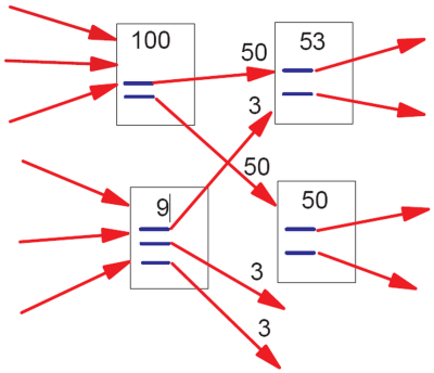
“In the image above, the lower-left document has “nine points of PageRank” and three outgoing links. The resulting PageRank flow along each outgoing link is consequently nine divided by three = three points of PageRank.
That simplistic model doesn’t work perfectly, however. Imagine if there were a loop:
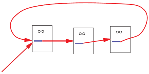
No PageRank would ever escape from the loop, and as incoming PageRank continued to flow into the loop, eventually the PageRank in that loop would reach infinity. Infinite PageRank isn’t that helpful [smiley face] so Larry and Sergey introduced a decay factor–you could think of it as 10-15% of the PageRank on any given page disappearing before the PageRank flows along the outlinks. In the random surfer model, that decay factor is as if the random surfer got bored and decided to head for a completely different page.”
Seems like a reasonable model?
Bad math
Reading about the “decay factor” trick made me laugh. I am imagining the two Google guys thinking: “OK, we are getting
 … …
But it goes to infinity! What to do, what to do? Eureka! Let’s make the sequence into
 …, …,
i.e., a geometric progression!” (Even though this step is mathematically silly, I have to admit that the explanation, “the bored surfer”, is brilliant! Post hoc?)
Now, what should be? Of course, they remember calc2 and know that the “ratio” should be less than  if you want the series to converge. if you want the series to converge.
“Let’s pick  ! Why? What do you mean why? This is the most natural choice!” ! Why? What do you mean why? This is the most natural choice!”
This number is a made-up parameter in the sense that there is no justification for choosing it over another value.
Of course, if the ordering that PageRank produces is independent from the choice of then we are OK.
When I tried to find such a theorem, I got nothing. Then I started to realize that there can’t be such a theorem. First, if there was, the only reason to choose a number over another would be the speed of convergence of the algorithm (.84 is better than .85). Second, the “naive” PageRank ( ) could serve as a counterexample. To confirm my hunch I did some literature search and quickly discovered this paper (and others): Bressan and Peserico Choose the damping, choose the ranking? J. Discrete Algorithms 8 (2010), no. 2, 199–213. To quote: ) could serve as a counterexample. To confirm my hunch I did some literature search and quickly discovered this paper (and others): Bressan and Peserico Choose the damping, choose the ranking? J. Discrete Algorithms 8 (2010), no. 2, 199–213. To quote:
“We prove that, at least on some graphs, the top  nodes assume all possible nodes assume all possible  orderings as the damping factor varies, even if it varies within an arbitrarily small interval (e.g. [0.84999, 0.85001]).” orderings as the damping factor varies, even if it varies within an arbitrarily small interval (e.g. [0.84999, 0.85001]).”
PageRank is often described as “elegant”. However, pulling a parameter from your ear is not only a very poor taste mathematically, it’s bad science. It’s similar to creating a mathematical theory of, say, planetary motion and deciding that the gravitational constant should be equal to, well,  . And why not? You do get a valid mathematical theory! Or, how about . And why not? You do get a valid mathematical theory! Or, how about  equal to ? equal to ?
There are of course other problems with PageRank. For example, there is an example of such a graph that changing a single link completely reverses the ranking (Ronny Lempel, Shlomo Moran: Rank-Stability and Rank-Similarity of Link-Based Web Ranking Algorithms in Authority-Connected Graphs. Inf. Retr. 8(2): 245-264 (2005)).
Consequences of bad math
There is a lot of mathematics in computational science, algorithms, software etc. It’s tempting to make math stuff up just because you can. The consequences are dare.
There is nothing more practical than a good theory. Conversely, a bad theory makes things based on it very impractical.
This is you: “My car is great: a powerful engine, excellent mileage, leather interior, etc. I love it!”

You don’t mind the bumpy ride? “What bumpy ride? Aren’t all cars supposed to run like this?”

So, you haven’t figured out the right shape (the math) for your wheels and you pay the price.
Worldwide suffering
Wikipedia: “the PageRank concept has proven to be vulnerable to manipulation, and extensive research has been devoted to identifying falsely inflated PageRank and ways to ignore links from documents with falsely inflated PageRank.”
In particular, (semi-)closed communities represent a problem. Linkfarms is the main example. Also, groups of hotels have a lot links to each other, but very few links to the rest of the web. The issue is that once the random surfer gets into one of such communities he can’t get out, adding more and more to the community’s PageRank.
Finding such communities of web pages, if they try to avoid detection, is an NP-hard problem (read “hard”). The answer from Google and others is to employ secret heuristics that identify these communities and then penalize their PageRank.
The result is numerous false positives that hurt legitimate sites and false negatives that rank linkfarms higher in the search results. In addition, the secrecy and the constant tweaking make the risks unmanageable for web-based businesses. It’s a mess.
To summarize, this is the sequence of events:
- the initial model produces meaningless results;
- they come up with an ad hoc fix;
- the model is still mathematically bad;
- the model becomes dominant nonetheless;
- now we’re all screwed.
There will always be bad math out there. What makes this a real abomination is the magnitude of the problem, i.e., Google. As a mathematician I find it disturbing that one piece of bad mathematics affects just about every Internet user in the world.
Did I justify the harsh language that I used here? You’ll be the judge of that.
Meanwhile what is the right way of ranking sites based on links? I’ll write a post about that in the near future. Short version: remove all “cycles”.
This is an excerpt from a longer article about PageRank.
Follow-ups: here and here.
Comments Off
May 21, 2011
MicroConf will be held in Las Vegas June 6th and 7th. It is “focused on self-funded startups and single founder software companies”. I’ve never been to a conference like that, i.e., non-academic, and the list of speakers looks very impressive.
If you plan to attend and want to chat, email me.
Comments Off
Next Page » |
|
|