Computer Vision & Math contains: mathematics courses, covers: image analysis and data analysis, provides: image analysis software. Created and run by Peter Saveliev.
Discrete differential forms
From Computer Vision and Math
Discrete differential forms... Why do we need them?
Suppose we have a function, $f$, that we know only as a "sampled" function, i.e, we only know its values at, say, 0, 1, 2, 4, 5 (in green below). Suppose that the derivative, $f'$, of the function is also sampled (purple).
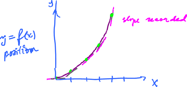
For example, $f$ might be the position, $f'$ the velocity. It's like you look at your odometer and speedometer once in a while, so that you measure the position and velocity at equal intervals. Then we have $g$ and $g^*$, which we may call "discrete functions":

Then it would make sense if $g^*$ was the derivative of $g$, in some way.
Question: How can we establish this relation this without actual differentiation?
Answer: we use the Fundamental Theorem of Calculus.
For the integral we use the Riemann integral, as follows: $$g(4)-g(0) \stackrel{?}{=} \displaystyle\int_0^4 g^*(x) dx.$$ Here the right hand side is the displacement. To integrate, let's turn $g^*$ into a step function.
By example, $$g(1)-g(0) \approx 1$$ but $$\displaystyle\int_0^1 g^*(x)dx = \displaystyle\int_0^1 0 dx = 0.$$ The right side only approximates the integral, so, in general, there is a mismatch.
Then the laws of physics are in danger as they are satisfied only approximately...
Next, if the sampling is improved by taking more sample values (we look at the dials more often), then the Riemann sums converge to the Riemann integral.
That's a good news.
However, we still have an issue to deal with.
Question: What about convergence? Suppose $f_n \rightarrow f$, does it mean that $f_n' \rightarrow f'$?
Answer: No.
As an example, consider the famous Weierstrass function: $$f(x) = \displaystyle\sum_{n=0}^{\infty} a^n cos(b^n \pi x); 0 < a < 1.$$ This series converges uniformly, so $f$ is continuous. But if $b > 1 + \frac{a}{2} \pi$, $f$ is nowhere differentiable.
So what do we do?
Idea: build the discrete calculus via discrete differential forms that mimic the smooth forms.
What if we choose, for $g^*$, secant lines instead of tangent lines?

Then
- 1) $g$ is the sampled $f$, as before, but
- 2) $g^*$ is the slopes on the secant lines.
Now the key step. Where should $g^*$ be defined?
Rather then defining $g^*$ at the end point of the intervals (0, 1, 2...), as $g$, we "expand" $g^*$ to the intervals, as a step function (purple): $g(x)=0$ on $(0,1)$, $g(x)=1$ on $(1,2)$, etc.
Then the fundamental theorem of calculus works!
Indeed:
$$\begin{align*} g(1)-g(0) &= \displaystyle\int_0^1 g^*(x) dx {\rm \hspace{6pt} --> match!} \\ 0 &= 0 \end{align*}$$
$$\begin{align*} g(2)-g(1) &= \displaystyle\int_1^2 g^*(x) dx {\rm \hspace{6pt} --> match!} \\ 1 &= 2-1 \end{align*}$$
It works because there is no approximation. It's like we have decided not to look at the odometer at all!
This is what we end up with:
| $g$ | $g^*$ | |
| $\{0, 1, 2, 3\}$ | $(0,1),(1,2),(2,3)$ | $\leftarrow$ the domain |
| points | intervals | $\leftarrow$ nature of the domain |
| $0$ | $1$ | $\leftarrow$ dimension of the domain |
| $0$-form | $1$-form | $\leftarrow$ terminology |
Note: they are undefined outside the domains, unlike smooth differential forms.
Informally, a discrete $k$-form is a differential form, the coefficients of which are constant on open $k$-cells (as in $5 dx$ rather than $x dx$).
Recall this about smooth forms in ${\bf R}^3$:
| $0$-forms: | a function $A$ |
| $1$-forms: | $\varphi = A dx + B dy + C dz$, the dot product $(A,B,C) \cdot (dx,dy,dz)$ (only $A dx + B dy$ in ${\bf R}^2$) |
| $2$-forms: | $\varphi = A dx \hspace{1pt} dy + B dy \hspace{1pt} dz + C dz \hspace{1pt} dx$ (only $A dx \hspace{1pt} dy$ in ${\bf R}^2$) |
| $3$-forms: | $\varphi = A dx \hspace{1pt} dy \hspace{1pt} dz$ (only $0$ in ${\bf R}^2$) |
Now, discrete forms are no different except there will be restrictions on $A, B, C$.
The $dx$, $dy$, $dz$ definition is an algebraic representation of the following formal definition.
Axioms (definition). Suppose $R$ is a region in ${\bf R}^3$. A differential $k$-form in ${\bf R}^3$ is a function ("functional") $$\varphi \colon R \times {({\bf R}^3)}^k \rightarrow {\bf R},$$ $$\varphi (x,y,z,dx, dy, dz)= r \in {\bf R},$$ with these properties on each ${\bf R}^3$ (note, $x,y,z$ correspond to $R$ and $dx, dy, dz$ correspond to ${({\bf R}^3)}^k)$:
- 1) Multilinearity:
- $\varphi(\cdot, b, c)$ is linear,
- $\varphi(a, \cdot, c)$ is linear,
- $\varphi(a, b, \cdot)$ is linear.
Note: $\varphi$ is a $3$-form, and $a,b,c \in {\bf R}^3$ ($x,y,z$ omitted here)
- 2) Antisymmetry:
- $\varphi(x,y,z) = -\varphi(y,x,z),$
- $\varphi(x,y,z) = -\varphi(x,z,y),$
- $\varphi(x,y,z) = -\varphi(z,y,x).$
A connection of discrete forms to this definition will be made later, via integration of cochains.
Geometric interpretation
What is the main difference?
The grid: the Euclidean space is divided into small, disjoint parts.
In dimension 1, these parts are: points and intervals.

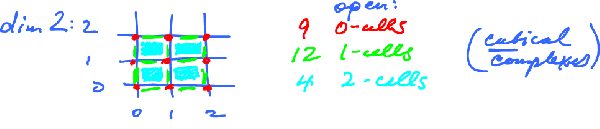
In dimension 2, these parts are: points, intervals, and squares.
For more see Cubical complexes.
Specifically, in dimension 2 we have:
- $0$-cells: $\{(0,0)\}, \{(0,1)\}, \ldots,$
- $1$-cells: $(0,1) \times 0$, $0 \times (0,1),\ldots,$
- $2$-cells: $(0,1) \times (0,1),\ldots.$
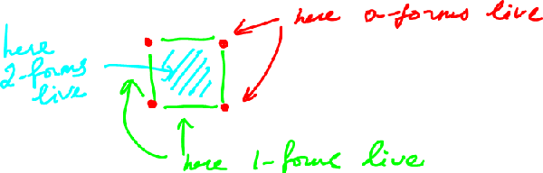
A $k$-form is defined on $k$-cells, only. As follows:
Examples of forms:
| dimension | forms defined on | graphical representation of forms | algebra (forms as cochains) |
| dim $1$ | $0$-cells | 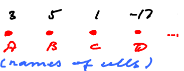 (a $0$-form) (a $0$-form)
| $\varphi(A)=3$, $\varphi(B)=5, \ldots$ |
| dim $1$ | $1$-cells | 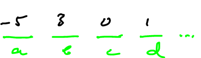 (a $1$-form) (a $1$-form)
| $\psi(a)=5$, $\psi(b)=3, \ldots$ |
| dim $2$ | $0$-cells | 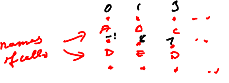 (a $0$-form) (a $0$-form)
| $\varphi(A)=0$, $\varphi(B)=1, \ldots$ |
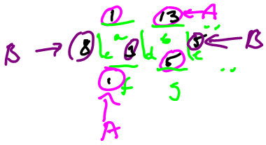
| dim $2$ | $1$-cells | 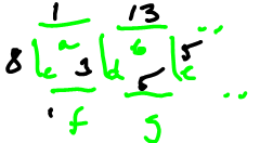 (a $1$-form) (a $1$-form)
| $\psi(a)=1$, $\psi(c)=8, \ldots$ |
| dim $2$ | $2$-cells | 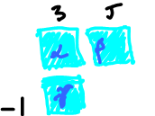 (a $2$-form) (a $2$-form)
| $\theta(\alpha)=3$, $\theta(\beta)=5, \ldots$ |
Observe that in the right column we no longer interpret the discrete forms as defined on points of each cell (constant) but simply as defined on each cell itself. This is called the cochain representation discussed later.
This is how we can connect this definition to the traditional representation of differential forms. We use the fundamental theorem of calculus for evaluation:
Given $\psi(a)=1$, then $\psi=1 dx$ on $a$.
Given $\psi(c)=8$, then $\psi = 8 dy$ on $c$.
Etc.
Example: $\psi = A dx + B dy$, where $A,B$ are functions defined on $1$-cells:
See next Algebra of discrete differential forms.
Digital discoveries
- Casinos Not On Gamstop
- Non Gamstop Casinos
- Casino Not On Gamstop
- Casino Not On Gamstop
- Non Gamstop Casinos UK
- Casino Sites Not On Gamstop
- Siti Non Aams
- Casino Online Non Aams
- Non Gamstop Casinos UK
- UK Casino Not On Gamstop
- Non Gamstop Casino UK
- UK Casinos Not On Gamstop
- UK Casino Not On Gamstop
- Non Gamstop Casino UK
- Non Gamstop Casinos
- Non Gamstop Casino Sites UK
- Best Non Gamstop Casinos
- Casino Sites Not On Gamstop
- Casino En Ligne Fiable
- UK Online Casinos Not On Gamstop
- Online Betting Sites UK
- Meilleur Site Casino En Ligne
- Migliori Casino Non Aams
- Best Non Gamstop Casino
- Crypto Casinos
- Casino En Ligne Belgique Liste
- Meilleur Site Casino En Ligne Belgique
- Bookmaker Non Aams
- カジノ ライブ
- онлайн казино с хорошей отдачей
- スマホ カジノ 稼ぐ
- ブック メーカー オッズ
- Top 3 Nhà Cái Uy Tín Nhất
- Trang Web Cá độ Bóng đá Của Việt Nam
- Casino En Ligne Avis
- Casino En Ligne France
- Casino En Ligne
- 꽁머니 토토
- Casino Online Non Aams
- Migliori Casino Non AAMS
- Meilleur Casino En Ligne
- Casino En Ligne France Légal
- Casino En Ligne France Légal
- Casinos En Ligne
- Mejores Casinos Online
